Not every search starts in an editor. run_app() opens a
local Shiny app that drives the whole scopusflow workflow through a
browser tab, from describing a search to exporting the records, without
writing any R. It runs on your own machine, so your Scopus key never
leaves it and requests come from your own network. The app doubles as a
way into the package itself, because it mirrors every choice you make
back as a runnable R script. Anything you can do in the app you can also
do from code, and the script panel shows you how.
This article describes the app without running it, since that would need a live server, so the code chunks are shown but not evaluated. The screenshots were taken from the running app with Demo mode left on, which needs no key and no network, so everything they show can be reproduced on your own machine in a minute.
Launching the app
The app needs the suggested packages shiny, bslib and callr, and ggplot2 for the plots. With those installed, one call opens it.
By default it listens only on 127.0.0.1, so it is
reachable from your own machine alone, and it opens your browser at the
address it prints. Passing launch.browser = FALSE leaves
the browser to you, and port fixes the port when you need a
stable address.
Demo mode
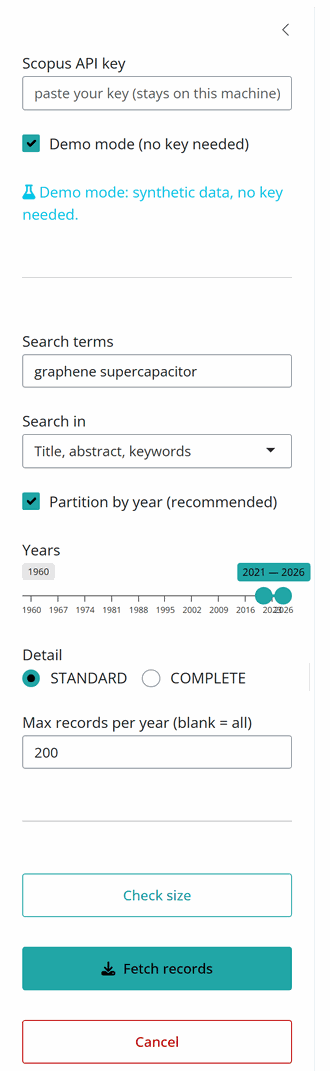
Demo mode is switched on when the app opens, so you can walk the
whole flow with no key at all. With it on, the harvest is simulated, the
live terminal still streams its per-cell progress, the tables and plots
still render, and the Compare topics tab still draws a figure. It is the
quickest way to learn where each control sits before you spend any
quota. The records come from example_records, the corpus of
138 real journal articles the package bundles because Scopus records may
not be redistributed, so every panel is exercised on real titles, DOIs,
journals and citation counts, and the by-year chart shows a real
publication curve with the shape the literature actually has. That
corpus spans 2015 to 2024, so a year range reaching outside it is drawn
from the nearest year it holds. Only the topic comparison is
synthesised, since it counts whole literatures, which no set of records
in hand can answer for. When you are ready for real results, paste your
Scopus key into the field at the top of the sidebar and switch Demo mode
off. The key stays in the running session and is never written into the
generated script.
Describing and sizing a search
The sidebar is where you describe the search. You enter your terms,
choose which field to search in, set a year range, and pick the level of
detail. Partitioning by year is recommended and switched on by default,
because it keeps each cell under the API’s offset ceiling, the same
reasoning behind a partitioned scopus_plan() in code. Check
size runs a cheap count first, the same one scopus_count()
performs, so you can see how much a query would retrieve before
committing to it. In demo mode it reports instead how many records it
would draw from the bundled corpus.
Fetching, with a live terminal
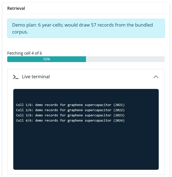
Fetch records starts the harvest in a background process, so the app
stays responsive while it works. The Live terminal panel tails the
worker’s output, streaming a line as each year-cell completes, and a
progress bar tracks how far through the plan the run has reached. Cancel
ends the background process at once, which does abandon whatever cell
was in flight. Every cell that had already finished was checkpointed as
it completed, and a checkpoint is written to a temporary file and
renamed into place, so a cancelled run leaves the cache whole and a
later run resumes from it. Internally the app builds a
scopus_plan() from your choices and hands it to
scopus_fetch_plan() with a cache directory and resume
turned on, so an interrupted or quota-limited run picks up where it left
off.
The reproducible code panel
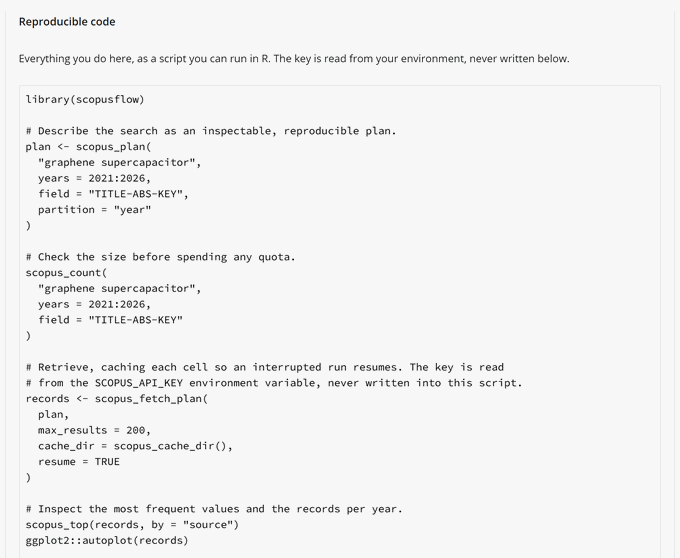
The Reproducible code panel is what turns the app into a tutorial. It
mirrors every choice you make, the query, the field, the years, whether
you partition by year, and the Compare topics options, and rewrites a
runnable R script as you go. Change a control and the script updates at
once, so you can see exactly which argument each choice sets. The key
never appears in the script. The panel notes that it is read from the
SCOPUS_API_KEY environment variable, so a script you share
carries the method but not your credentials. Download script saves
exactly what you see.
Reading the results
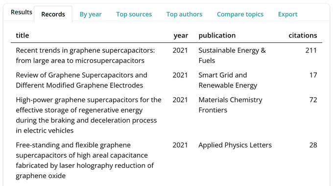
When the run finishes, the Results tabs come to life. Records shows a
table of titles, years, sources and citations. By year draws the
publications-per-year trend through autoplot(). Top sources
and Top authors tally the most frequent of each with
scopus_top() and plot_scopus_top(). Every
figure is drawn by the same library functions you would call from a
script, so the app shows you nothing you could not reproduce.
Comparing topics
The Compare topics tab asks a different question from a harvest. It
retrieves no records at all, and measures instead how a set of
sub-topics co-occur with your search over time, as a share of it, with
your search terms acting as the reference topic. You enter
comma-separated comparison terms, optionally pick one to highlight, and
toggle the stability band and whether record counts appear on the
labels. Because each term needs one count request per year, the tab
shows how many requests a comparison will make and warns when the grid
grows large. In demo mode the comparison is synthesised so you can see
the figure offline. With a key it calls
scopus_compare_topics() and draws the result with
plot_scopus_comparison(), the same figure the package
produces, and a Comparison download saves the underlying numbers as a
CSV.
Exporting
Every result the app shows comes with one-click export. The records
can be saved as an RDS file, as a clean DOI list, and as BibTeX and RIS
for a reference manager such as Zotero or EndNote, drawn from
as_bibtex() and as_ris(), and as a PRISMA-S
search record in Markdown, drawn from
scopus_search_report(). In demo mode that record carries no
plan or retrieval time, and says so, since the records on screen were
replayed from the bundled corpus and never retrieved. The comparison can
be saved as a CSV. None of this contacts the API again, because it works
on results already in hand. Between the downloaded script and the
exported records, a session in the app leaves you with both the data and
the code that produced it.
Beyond the app
Anything you can do in the app you can also do from code, but the
reverse does not hold. The app covers planning, retrieval and the trend,
top and comparison analyses, and the package goes further.
scopus_intersections() counts how a set of named concepts
and their intersections overlap in the literature, and
plot_scopus_intersections() draws the result.
scopus_abstract() retrieves abstract text and richer
metadata than the Search API returns, and scopus_corpus()
builds on it to give a harvest author keywords and structured references
for tools further downstream. When a session in the app has taken you as
far as it goes, the downloaded script is the place to carry on from.