This vignette is fully reproducible without a Scopus API key. It draws on a small static fixture bundled with the package, so the whole workflow can be shown offline. The few steps that genuinely need the API are shown but not run.
Describing a search as a plan
A plan separates describing a search from executing it. Plans are
inspectable, saveable and version-controllable, and they can be
partitioned, for example by year, so that a large retrieval stays under
the API’s start < 5000 ceiling and can be cached and
resumed.
plan <- scopus_plan(
  "machine translation",
  years     = 2018:2020,
  field     = "TITLE-ABS-KEY",
  partition = "year"
)
plan
#> <scopus_plan> (3 cells, view "STANDARD", partition "year")
#> # A tibble: 3 × 6
#>    cell query                              date   year view     page_size
#> * <int> <chr>                              <chr> <int> <chr>        <int>
#> 1     1 TITLE-ABS-KEY(machine translation) 2018   2018 STANDARD       200
#> 2     2 TITLE-ABS-KEY(machine translation) 2019   2019 STANDARD       200
#> 3     3 TITLE-ABS-KEY(machine translation) 2020   2020 STANDARD       200
Each row is one query cell. Field tags wrap the query and years become a date filter:
scopus_plan("language learning", field = "TITLE")$query
#> [1] "TITLE(language learning)"
scopus_plan("x", years = 2015:2020)$date
#> [1] "2015-2020"
Sizing and fetching
With a key configured, you size a search cheaply and then execute the plan, optionally caching each cell so that an interrupted run resumes without re-spending quota. These contact the API, so they are not evaluated here:
scopus_count("machine translation", years = 2018:2020, field = "TITLE-ABS-KEY")

records <- scopus_fetch_plan(plan, cache_dir = scopus_cache_dir(), resume = TRUE)
The record schema
Whether records come from the API or from the bundled example data, they share one stable schema. The package ships a small, already normalised set, which we use here to continue offline:
records <- example_records
records
#> <scopus_records> 6 records
#> query: "illustrative multi-disciplinary sample"
#> # A tibble: 6 × 9
#>   entry_number scopus_id   doi   title authors  year date  publication citations
#>          <int> <chr>       <chr> <chr> <chr>   <int> <chr> <chr>           <int>
#> 1            1 85000000001 10.1… Geno… Zhang …  2019 2019… Nature            540
#> 2            2 85000000002 10.1… Deep… Kumar …  2020 2020… Nature            210
#> 3            3 85000000003 10.1… Clim… Okafor…  2018 2018… Nature Cli…       122
#> 4            4 85000000004 10.1… Grap… Tanaka…  2021 2021… Advanced M…        45
#> 5            5 85000000005 10.1… Chec… Garcia…  2020 2020… The Lancet…       388
#> 6            6 85000000006 10.1… Obse… Abbott…  2016 2016… Physical R…      4200
scopus_records() produces this same shape from a raw API
response, flattening the nested result into one row per record.
DOIs and change tracking
Extract a clean, deduplicated DOI list for import into a reference manager, and compare two retrievals to see exactly what changed:
dois <- scopus_extract_dois(records)
dois
#> [1] "10.1038/s41586-019-0001-1"      "10.1038/s41586-020-0002-2"
#> [3] "10.1038/s41558-018-0085-1"      "10.1002/adma.202100001"
#> [5] "10.1016/S1470-2045(20)30013-9"  "10.1103/PhysRevLett.116.061102"

# Suppose a later retrieval added one DOI and dropped another.
later <- c(dois[-1], "10.1000/example.999")
scopus_diff_dois(old = dois, new = later)
#> <scopus_doi_diff> 1 added, 1 removed, 5 unchanged
#> # A tibble: 7 × 2
#>   doi                            status
#>   <chr>                          <fct>
#> 1 10.1000/example.999            added
#> 2 10.1038/s41586-019-0001-1      removed
#> 3 10.1002/adma.202100001         unchanged
#> 4 10.1016/S1470-2045(20)30013-9  unchanged
#> 5 10.1038/s41558-018-0085-1      unchanged
#> 6 10.1038/s41586-020-0002-2      unchanged
#> 7 10.1103/PhysRevLett.116.061102 unchanged
You can write the DOIs to a path you specify:
out <- file.path(tempdir(), "dois.csv")
scopus_extract_dois(records, file = out)
readLines(out)
#> [1] "\"doi\"" "\"10.1038/s41586-019-0001-1\""
#> [3] "\"10.1038/s41586-020-0002-2\"" "\"10.1038/s41558-018-0085-1\""
#> [5] "\"10.1002/adma.202100001\"" "\"10.1016/S1470-2045(20)30013-9\""
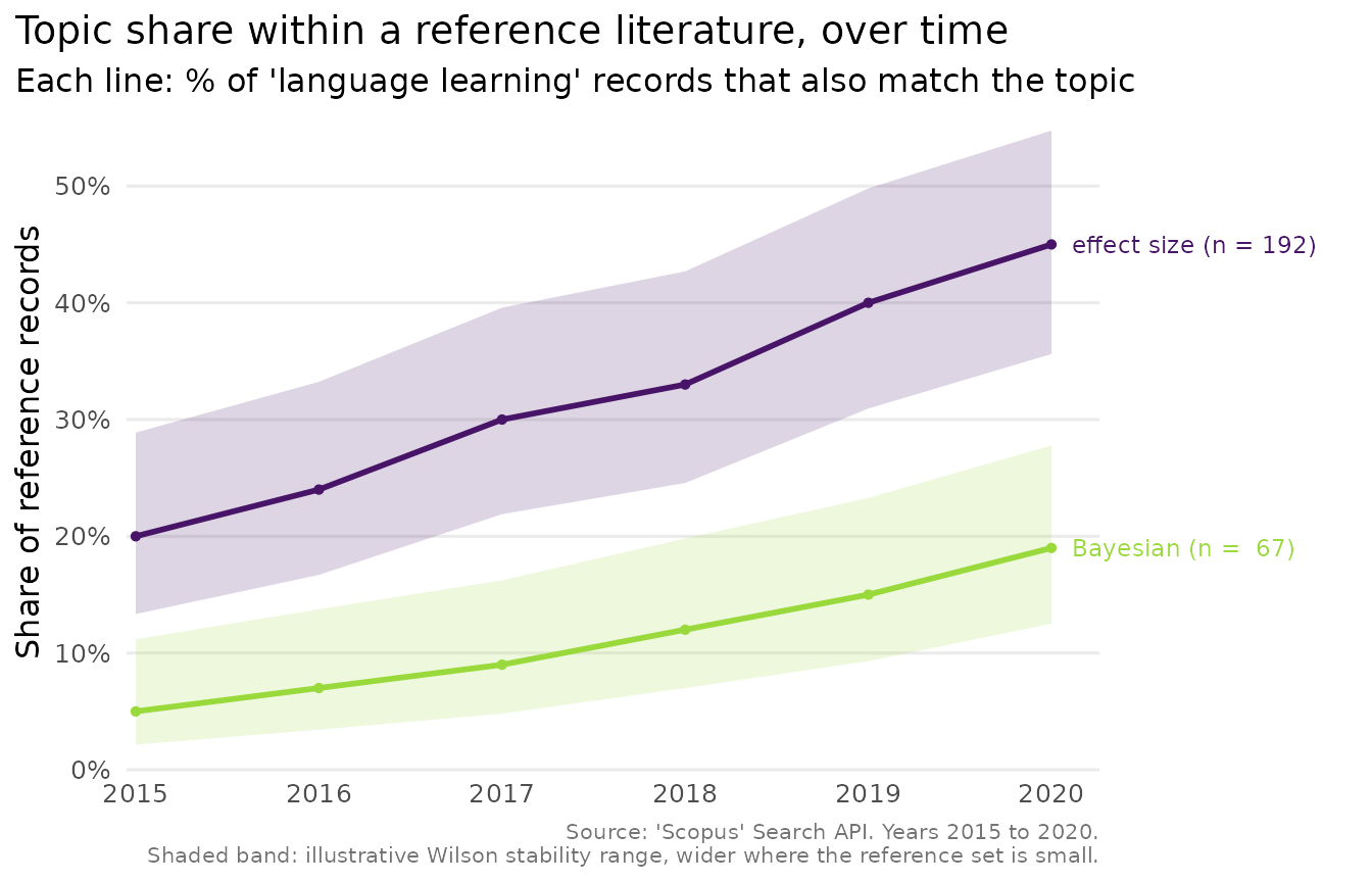
#> [7] "\"10.1103/PhysRevLett.116.061102\""Comparing topic trends
scopus_compare_topics() issues one count request per
term per year, so it needs the API. Its output has a fixed shape, which
we reproduce here to show the plot:
cmp <- scopus_compare_topics(
  reference_query  = "language learning",
  comparison_terms = c("effect size", "Bayesian"),
  years            = 2015:2020,
  field            = "TITLE-ABS-KEY"
)
# A stand-in comparison object with the same columns scopus_compare_topics()
# returns, so the plotting step is reproducible offline.
cmp <- tibble::tibble(
  query = "q",
  query_type = rep(c("reference", "comparison", "comparison"), each = 6),
  abridged_query = rep(c("language learning", "effect size", "Bayesian"), each = 6),
  year = rep(2015:2020, 3),
  n = c(rep(100, 6), 20, 24, 30, 33, 40, 45, 5, 7, 9, 12, 15, 19),
  reference_n = rep(100, 18),
  comparison_percentage = c(rep(100, 6), 20, 24, 30, 33, 40, 45, 5, 7, 9, 12, 15, 19),
  average_comparison_percentage = rep(c(100, 32, 11.2), each = 6)
)
class(cmp) <- c("scopus_comparison", class(cmp))
cmp
#> <scopus_comparison> (3 topics)
#> # A tibble: 18 × 8
#>    query query_type abridged_query  year     n reference_n comparison_percentage
#>    <chr> <chr>      <chr>          <int> <dbl>       <dbl>                 <dbl>
#>  1 q     reference  language lear…  2015   100         100                   100
#>  2 q     reference  language lear…  2016   100         100                   100
#>  3 q     reference  language lear…  2017   100         100                   100
#>  4 q     reference  language lear…  2018   100         100                   100
#>  5 q     reference  language lear…  2019   100         100                   100
#>  6 q     reference  language lear…  2020   100         100                   100
#>  7 q     comparison effect size     2015    20         100                    20
#>  8 q     comparison effect size     2016    24         100                    24
#>  9 q     comparison effect size     2017    30         100                    30
#> 10 q     comparison effect size     2018    33         100                    33
#> 11 q     comparison effect size     2019    40         100                    40
#> 12 q     comparison effect size     2020    45         100                    45
#> 13 q     comparison Bayesian        2015     5         100                     5
#> 14 q     comparison Bayesian        2016     7         100                     7
#> 15 q     comparison Bayesian        2017     9         100                     9
#> 16 q     comparison Bayesian        2018    12         100                    12
#> 17 q     comparison Bayesian        2019    15         100                    15
#> 18 q     comparison Bayesian        2020    19         100                    19
#> # ℹ 1 more variable: average_comparison_percentage <dbl>
if (requireNamespace("ggplot2", quietly = TRUE)) {
  plot_scopus_comparison(cmp)
}
Export and interoperability
Hand results to bibliometrix-style workflows, or save
and reload them:
head(as_bibliometrix(records))
#>          AU                                                                 TI
#> 1  ZHANG F.       GENOME EDITING WITH CRISPR-CAS9: PRINCIPLES AND APPLICATIONS
#> 2  KUMAR S.                 DEEP LEARNING FOR MEDICAL IMAGE ANALYSIS: A REVIEW
#> 3 OKAFOR N.                    CLIMATE CHANGE ADAPTATION IN COASTAL MEGACITIES
#> 4 TANAKA H.             GRAPHENE ELECTRODES FOR NEXT-GENERATION ENERGY STORAGE
#> 5 GARCIA M.                      CHECKPOINT INHIBITORS IN CANCER IMMUNOTHERAPY
#> 6 ABBOTT B. OBSERVATION OF GRAVITATIONAL WAVES FROM A BINARY BLACK HOLE MERGER
#>                        SO                             DI   PY   TC          UT
#> 1                  NATURE      10.1038/s41586-019-0001-1 2019  540 85000000001
#> 2                  NATURE      10.1038/s41586-020-0002-2 2020  210 85000000002
#> 3   NATURE CLIMATE CHANGE      10.1038/s41558-018-0085-1 2018  122 85000000003
#> 4      ADVANCED MATERIALS         10.1002/adma.202100001 2021   45 85000000004
#> 5     THE LANCET ONCOLOGY  10.1016/S1470-2045(20)30013-9 2020  388 85000000005
#> 6 PHYSICAL REVIEW LETTERS 10.1103/PhysRevLett.116.061102 2016 4200 85000000006
#>       DB
#> 1 SCOPUS
#> 2 SCOPUS
#> 3 SCOPUS
#> 4 SCOPUS
#> 5 SCOPUS
#> 6 SCOPUS

path <- file.path(tempdir(), "records.rds")
write_scopus_records(records, path)
identical(read_scopus_records(path), records)
#> [1] TRUE
Handling failures
Network and API problems surface as typed conditions, all inheriting
from scopus_error, so a workflow can respond to them in
code:
tryCatch(
  scopus_fetch("..."),
  scopus_error_no_key     = function(e) message("No API key configured."),
  scopus_error_rate_limit = function(e) message("Rate limited, so backing off."),
  scopus_error            = function(e) message("Scopus error: ", conditionMessage(e))
)