Analysing and visualising a literature

library(scopusflow)

Once a set of records is in hand, the package offers a small analysis layer that turns it into the figures a bibliometric study usually needs. The steps that contact the API are shown but not run; the rest use the bundled example_records and run offline.

What is in a record set

scopus_top() tallies the most frequent sources or authors. Author strings that hold several names are split, so each contributor is counted once per record.

scopus_top(example_records, by = "source")
#> # A tibble: 5 × 2
#>   value                       n
#> * <chr>                   <int>
#> 1 Nature                      2
#> 2 Advanced Materials          1
#> 3 Nature Climate Change       1
#> 4 Physical Review Letters     1
#> 5 The Lancet Oncology         1
scopus_top(example_records, by = "author", n = 5)
#> # A tibble: 5 × 2
#>   value         n
#> * <chr>     <int>
#> 1 Abbott B.     1
#> 2 Garcia M.     1
#> 3 Kumar S.      1
#> 4 Okafor N.     1
#> 5 Tanaka H.     1

plot_scopus_top(scopus_top(example_records, by = "source"))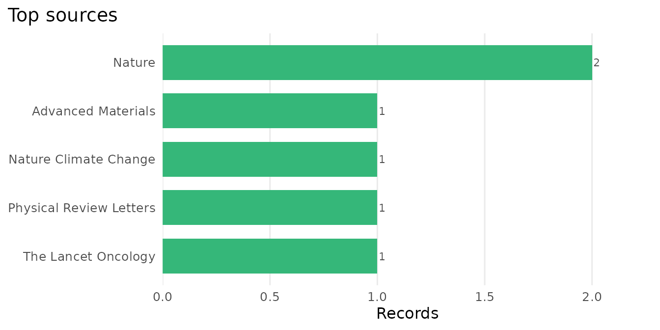

A record set also has an honest default view: autoplot() draws its records per year.

ggplot2::autoplot(example_records)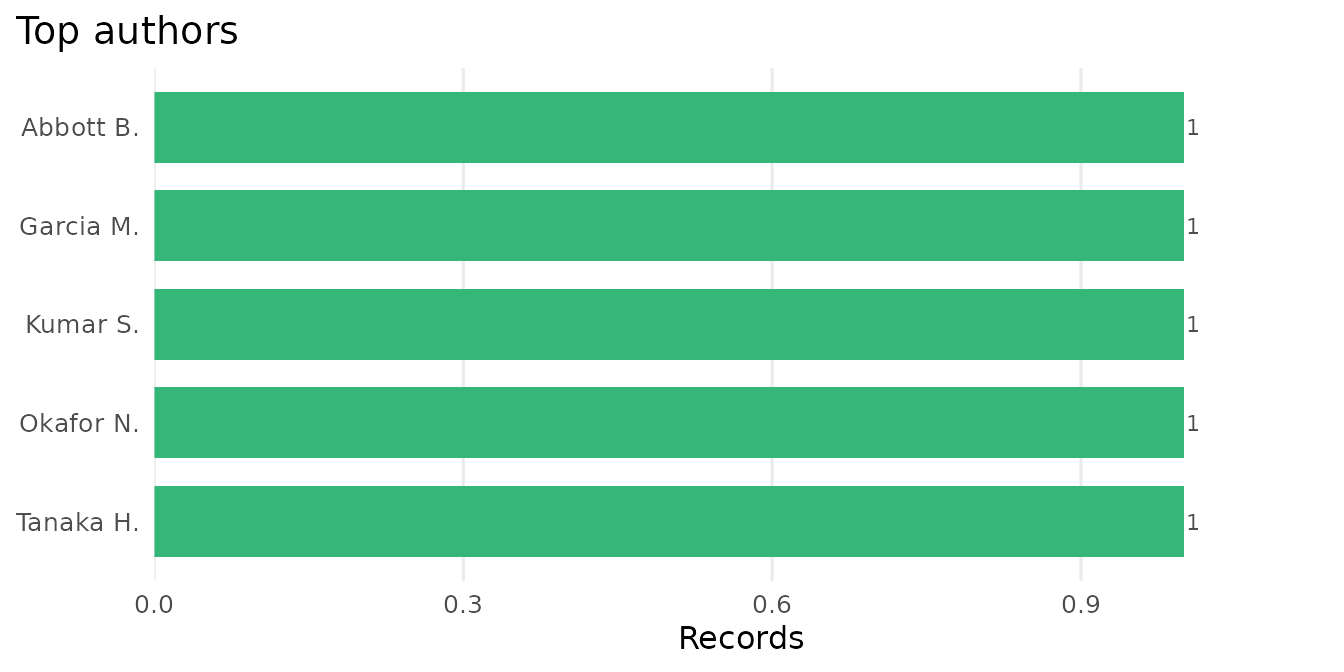

How a literature grows

scopus_trend() counts how many records match a query in each year, which is the size of a literature over time. It issues one count request per year, so it needs the API.

tr <- scopus_trend("graphene", years = 2004:2022, field = "TITLE-ABS-KEY")
plot_scopus_trend(tr)

The result has a fixed shape, which we reproduce here to show the plot.

years <- 2004:2022
tr <- tibble::tibble(query = "TITLE-ABS-KEY(graphene)", year = years,
                     n = round(exp(seq(log(50), log(28000), length.out = length(years)))))
class(tr) <- c("scopus_trend", class(tr))
plot_scopus_trend(tr)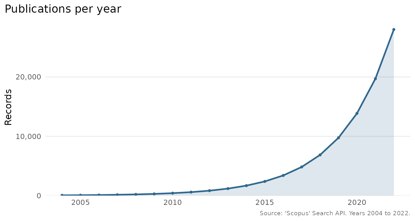

Reading the fuller record

The Search API returns a few fields per record. To read the abstract and the fuller metadata for a record you already know, scopus_abstract() calls the Abstract Retrieval API, by DOI or ‘Scopus’ identifier. A batch is resilient: an identifier that cannot be found yields a row of NAs with a warning rather than stopping the run.

ab <- scopus_abstract(c("10.1038/s41586-019-0001-1", "10.1103/PhysRevLett.116.061102"))
ab[, c("doi", "title", "year")]
substr(ab$abstract[1], 1, 200)

Beyond five thousand records

A single Search API query returns at most its first 5000 records under the ordinary offset paging. When you need the whole of a larger result set in one pass, scopus_fetch(cursor = TRUE) follows the API’s cursor instead, which has no such ceiling.

recs <- scopus_fetch("TITLE-ABS-KEY(microplastics)", cursor = TRUE)
nrow(recs)

The records then arrive in the API’s deep-paging order rather than sorted by relevance, which is the right trade for a complete harvest.