
depictr is a single, consistent toolkit of publication-ready plots that span the whole analysis workflow, from a first look at the data, through model estimates and predictions, to diagnostics, uncertainty and reporting. Most packages address one part of this work, whereas depictr aims to cover it from end to end with one theme, one palette and one set of label conventions. Every plotting function returns a ggplot2 object (or a patchwork for composite panels), so a plot can be refined further with the usual + syntax.
This is the R half of a sibling pair. The Python package of the same name covers most of the same workflow on top of plotnine. Its README lists the handful of functions that have yet to be ported and the differences that change what a figure shows, many of them arguments the Python functions do not yet take.
Gallery
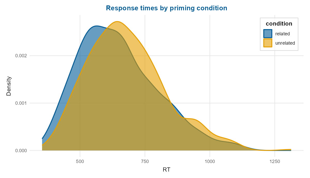
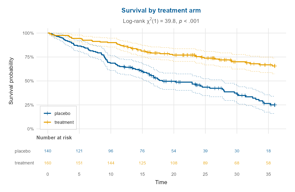
A grouped density (the default palette is a colourblind-safe set based on Okabe-Ito) and Kaplan-Meier survival curves with confidence bands and a number-at-risk table, each from a single function call:
Installation
depictr is on CRAN:
install.packages("depictr")The development version installs from GitHub:
# install.packages("remotes")
remotes::install_github("pablobernabeu/depictr")
What’s in the box
The functions fall into seven families that follow the analysis workflow. Exploratory plots and a descriptive summary table open it. The model-estimate views come next (forest plots, model comparison, predictions, interactions and random effects), then residual diagnostics with the standard classification curves, and then posterior summaries and power curves. Further families cover principal components, clustering and survival, time series, and the shared theme with the accessibility checks, composition, saving and reporting helpers. The reference lists every function by family.
Heavier modelling back-ends (lme4, broom, simr) are optional (in Suggests) and used only when present. The core functions, examples, tests and vignettes run on base lm/glm and the bundled data alone.
Measured accessibility
The default palette is the Okabe-Ito set, and that choice is checked. The package ships a simulator of colour-vision deficiency based on the model of Machado, Oliveira and Fernandes (2009), and palette_safety() measures how far apart the palette’s colours stay under each deficiency.
A safe palette is not a safe figure, though, so check_figure() audits the plot you are about to submit. It measures how separable the encoding colours are under each dichromacy and in greyscale, how small the text becomes at a stated output width, how well text and geometry contrast with their backgrounds under WCAG, and whether any distinction rests on colour alone. The size check covers the text drawn inside the panel as well as around it, and the contrast check covers the text around it alone. Each row reports the value it measured next to the threshold, so a verdict can be argued with. For a figure saved at its final width, give that width as both width_cm and render_width_cm, or neither, or let save_plot(check = TRUE) audit it at the width it saves. A journal that caps text size, as Nature does at 7 pt, can be held to its cap with max_text_pt.
check_figure(explore_distribution(lexical_decision, RT, group = condition),
             width_cm = 8.9)
The audit leaves continuous colour scales alone, and the colour rows of a heatmap say so. For those, prefer a perceptually ordered map such as viridis or the package’s sequential and diverging ramps.
Three limits of the palette are worth knowing. The colourblind-safety guarantee covers the eight base colours, and past those the palette interpolates, with a warning from depictr_palette(). The guarantee is also confined to hue confusion: in greyscale the palette’s orange and sky blue differ by only 0.79 in CIE lightness, so they print as the same grey. A figure that may be printed in black and white wants fewer groups, a sequential palette, or a redundant shape or line type. The palette also falls short on contrast. Four of the eight colours fall below the 3:1 against white that WCAG asks of a graphical object. The orange is one of them, and it is the second colour, so every default figure that colours two or more groups uses it. The example above therefore fails geometry_contrast, as well as redundant_encoding and, at 8.9 cm, text_size. Opaque marks, the vermillion #d55e00 in the orange’s place and a redundant shape or line type clear the two colour rows. scale_colour_depictr(order = "contrast") puts the vermillion there for one plot, and depictr_options(palette = depictr_palette(order = "contrast")) does so for every later one.
A first plot
library(depictr)

fit <- lm(yield ~ rainfall + fertiliser + soil_ph + treatment, data = crop_yield)
coefficient_plot(fit, order = "descending")
The Get started article walks through the whole workflow, from exploration to diagnostics and reporting.
Bundled data
Five reproducibly simulated datasets (lexical_decision, wellbeing_survey, crop_yield, clinical_trial and monthly_sales) ship with the package and power every example and vignette. Each is documented under its own name and described in the Get started article, and all are generated by data-raw/generate_datasets.R with fixed seeds.
Learn more
Each vignette takes one stretch of the workflow and works through it on the bundled data.
-
vignette("depictr"): getting started -
vignette("exploring-data"): exploratory plots, estimation statistics and tables -
vignette("model-estimates"): estimates, comparison, predictions, random effects and Bayesian posteriors -
vignette("diagnostics-and-uncertainty"): diagnostics, classification, posteriors, power -
vignette("multivariate-and-survival"): PCA, clustering with diagnostics, survival curves -
vignette("time-series"): trends, autocorrelation, decomposition, seasonality and forecasts
How depictr relates to other packages
depictr aims for breadth and consistency across the workflow, and it complements the specialised packages. Several of those remain the better choice for a deeper treatment of any one area, among them ggstatsplot (statistical details on plots), sjPlot and the easystats family (see, parameters, performance), marginaleffects / ggeffects (predictions), GGally (pairs), factoextra (PCA and clustering), survminer (survival), feasts / ggfortify (time series), ggdist / dabestr (distributions and estimation) and bayesplot / tidybayes (Bayesian). depictr offers one consistent default for all of these tasks within a single package.
Automated maintenance
depictr draws on a number of plotting and modelling packages, so scheduled GitHub Actions keep it healthy between releases. A daily job checks the package and its full test suite against both the current and the development versions of its dependencies, and a weekly job checks every URL in the documentation. On top of those, R CMD check runs on every push across Linux, macOS and Windows.
Citation
citation("depictr") gives the preferred reference. The DOI that CRAN assigned to the package is https://doi.org/10.32614/CRAN.package.depictr, and it covers every version. The About page carries the same citation with a BibTeX entry and a short note on the developer, and the repository ships CITATION.cff for the Cite this repository button on GitHub. The methods the package implements are cited in the relevant help pages and vignettes, drawing on a single bibliography at inst/REFERENCES.bib.
Licence
MIT (c) Pablo Bernabeu. See the licence.
Contributing
Issues and pull requests are welcome. The contributing guide describes the development setup and the conventions the package follows, and everyone taking part is asked to honour the Code of Conduct.