Plot the distribution of a variable

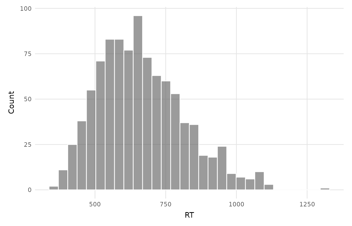
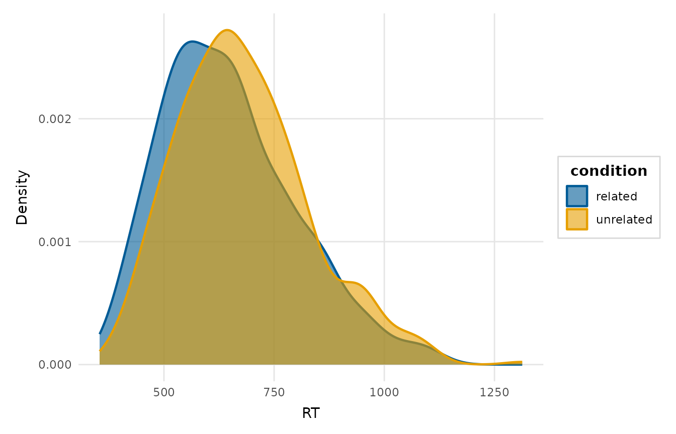
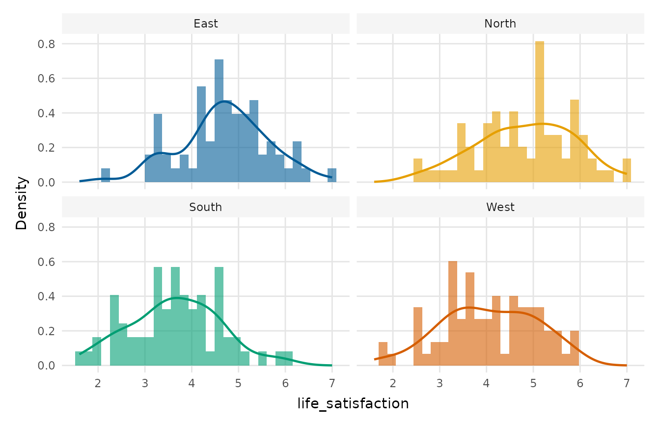
Draws a histogram, a density curve, or both, optionally split by a grouping variable. A quick first look at a continuous variable.

Usage

explore_distribution(
  data,
  x,
  group = NULL,
  type = c("histogram", "density", "both"),
  bins = 30,
  alpha = 0.6,
  position = NULL,
  palette = NULL,
  facet = FALSE,
  legend_inside = FALSE,
  title = NULL,
  x_lab = NULL
)

Arguments

data

A data frame.

x

The continuous variable to display. Either a string or an unquoted column name.

group

Optional grouping variable (string or unquoted name) mapped to colour/fill.

type

One of "histogram", "density" or "both".

bins

Number of histogram bins.

alpha

Fill transparency (useful when groups overlap).

position

Histogram position adjustment, e.g. "identity", "stack" or "dodge". The default (NULL) chooses "dodge" when group is set (so overlapping bars stay readable) and "identity" otherwise.

palette

Colours for the groups; defaults to depictr_palette().

facet

When a group is given, draw one panel per group instead of overlaying them. This is much clearer than an overlay once there are more than two or three groups (overlaid histograms in particular become hard to read). Defaults to FALSE. Ignored when there is no group.

legend_inside

When TRUE (and a group is given without facet), draw the colour legend inside the panel (in the top-right corner a unimodal histogram/density leaves empty) over a translucent background, instead of in a right-hand margin. Defaults to FALSE.

title, x_lab

Plot title and x-axis label (defaults to the variable name).

Value

A ggplot2::ggplot object.

Examples

explore_distribution(lexical_decision, RT)

explore_distribution(lexical_decision, RT, group = condition, type = "density")

# One panel per group keeps many groups legible:
explore_distribution(wellbeing_survey, life_satisfaction, group = region,
                     type = "both", facet = TRUE)