Plot frequentist and Bayesian estimates together — frequentist_bayesian

Presents the estimates from a frequentist model and a Bayesian model on one plot, with the two sources distinguished by the first two colours of the colourblind-safe depictr_palette() (brand blue and orange).

Usage

frequentist_bayesian_plot(
  frequentist,
  bayesian,
  conf_level = 0.95,
  labels = NULL,
  interaction = c("times", "asterisk", "colon", "space"),
  intercept = TRUE,
  facet = TRUE,
  scales = c("free", "fixed"),
  note_frequentist_no_prior = FALSE,
  vertical_line_at_x = 0,
  title = NULL,
  subtitle = NULL,
  x_lab = "Estimate",
  ...
)

Arguments

frequentist: A frequentist model (e.g. from lm, glm or lmerTest::lmer) or a tidy data frame of estimates.
bayesian: A Bayesian model, a posterior draws object, a draws matrix/data frame, or a tidy data frame of posterior summaries.
conf_level: Confidence/credible level for models.
labels, interaction, intercept: See compare_models(). intercept defaults to TRUE here, matching the original behaviour.
facet, scales: Layout controls. Because a Bayesian model almost always carries a large intercept alongside small slopes, the comparison defaults to a faceted, free-scaled layout (facet = TRUE): each term gets its own panel and free x-axis, so every posterior and its frequentist overlay stay legible. Pass facet = FALSE (or scales = "fixed") for the classic single shared-axis plot.
note_frequentist_no_prior: If TRUE, append "(no prior)" to the frequentist legend label, which is helpful when the title names the Bayesian prior.
vertical_line_at_x: Position of the vertical reference line (NA to omit).
title, subtitle, x_lab: Title, subtitle and x-axis label.
...: Further arguments passed to compare_models() on the summary path (ignored on the distribution path).

Value

A ggplot2::ggplot object.

Details

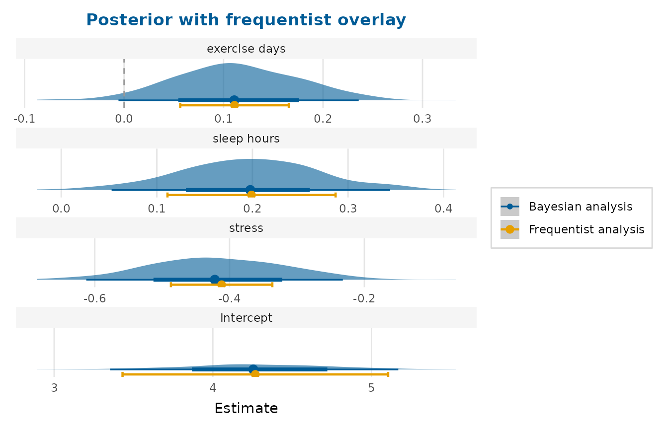
This is the modernised successor to the original frequentist_bayesian_plot() gist, which built on brms::mcmc_plot() to show the full Bayesian posterior with the frequentist estimate overlaid. 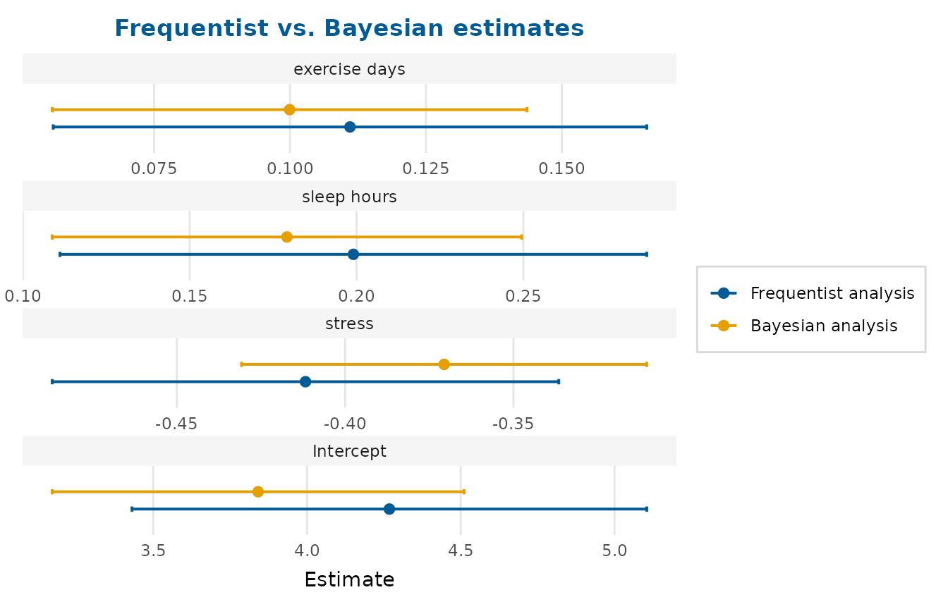That namesake behaviour is restored here: when bayesian carries posterior draws (a brms/rstanarm fit, a posterior draws object, a draws matrix, or a long/wide draws data frame), the full posterior distribution is drawn per term (a 'ggdist' half-eye) and the frequentist point and confidence interval is overlaid at the same position. When bayesian is only a tidy table of posterior summaries (columns such as term, estimate, conf.low/conf.high, or the Estimate, l-95% CI, u-95% CI of brms::fixef()), the function shows the familiar two-source forest plot via compare_models().

Terms are aligned by their canonical display label, so the brms-style b_ prefix is reconciled automatically against the frequentist term names.

Examples

# Summary path: a tidy "Bayesian" summary as a data frame. The summary here
# stands in for a regularised posterior, so a weakly informative prior pulls
# each estimate toward zero and narrows its interval; a real posterior would
# come from the model fit rather than from arithmetic on the frequentist one.
freq <- lm(life_satisfaction ~ stress + sleep_hours + exercise_days,
           data = wellbeing_survey)
bayes <- tidy_estimates(freq)
bayes$estimate <- bayes$estimate * 0.9
half <- (bayes$conf.high - bayes$conf.low) / 2 * 0.8
bayes$conf.low <- bayes$estimate - half
bayes$conf.high <- bayes$estimate + half
frequentist_bayesian_plot(freq, bayes,
                          title = "Frequentist vs. Bayesian estimates")


# Distribution path: simulated posterior draws (one column per term) drawn as
# full posteriors with the frequentist point + CI overlaid.
set.seed(1)
co <- coef(freq)
draws <- as.data.frame(lapply(co, function(m) rnorm(400, m, abs(m) * 0.1 + 0.05)))
names(draws) <- names(co)
frequentist_bayesian_plot(freq, draws,
                          title = "Posterior with frequentist overlay")