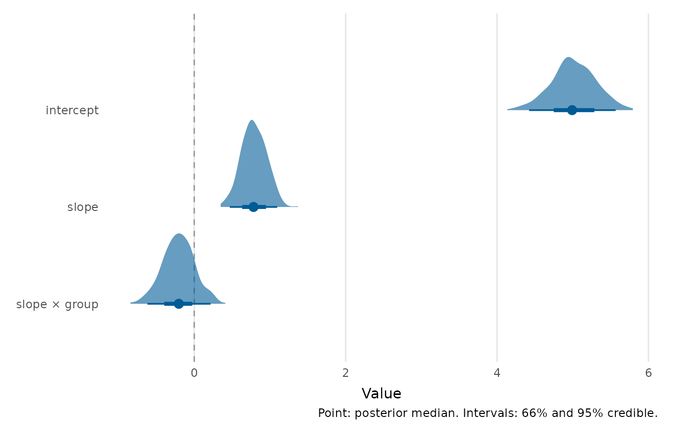
Plot posterior distributions — posterior

Displays posterior (or, more generally, bootstrap or simulation) draws as a distribution per parameter, in the style of a half-eye (a density slab with a point-and-interval beneath it), an interval-only forest plot, a gradient interval or a dotplot. The full shape of the posterior is shown, so skew, multimodality and the relative mass on either side of a reference value are all visible, rather than a point and two limits alone.

Usage

posterior_plot(
  draws,
  style = c("halfeye", "interval", "gradient", "dots"),
  point = c("median", "mean"),
  widths = c(0.66, 0.95),
  interaction = c("times", "asterisk", "colon", "space"),
  labels = NULL,
  reference_line = 0,
  rope = NULL,
  pd = FALSE,
  facet = FALSE,
  scales = c("fixed", "free"),
  colour = depictr_brand(),
  fill = depictr_brand(),
  rope_fill = depictr_reference(),
  rope_alpha = 0.15,
  title = NULL,
  x_lab = "Value",
  caption = NULL
)

Arguments

draws: Posterior draws: a fitted model (brms/rstanarm), a posterior draws object, a matrix, or a long/wide data frame (see Details).
style: One of "halfeye" (density slab + interval, the default), "interval" (point and two nested intervals, no slab), "gradient" (a colour-graded interval) or "dots" (a quantile dotplot). Unknown values and a missing 'ggdist' fall back to "interval".
point: Central summary: "median" or "mean".
widths: Two interval widths (inner and outer), as probabilities. The outer width is used for the caption and the displayed interval mass.
interaction: Passed to format_terms() for the parameter labels.
labels: Optional named character vector renaming parameters, e.g. c(conditionunrelated = "condition"). Unmatched parameters fall back to format_terms().
reference_line: Position of a vertical reference line, or NULL/NA to omit it. There is no universally meaningful reference for every parameter, so this defaults to 0 (the usual "no effect" line for differences and slopes) but should be set or cleared deliberately.
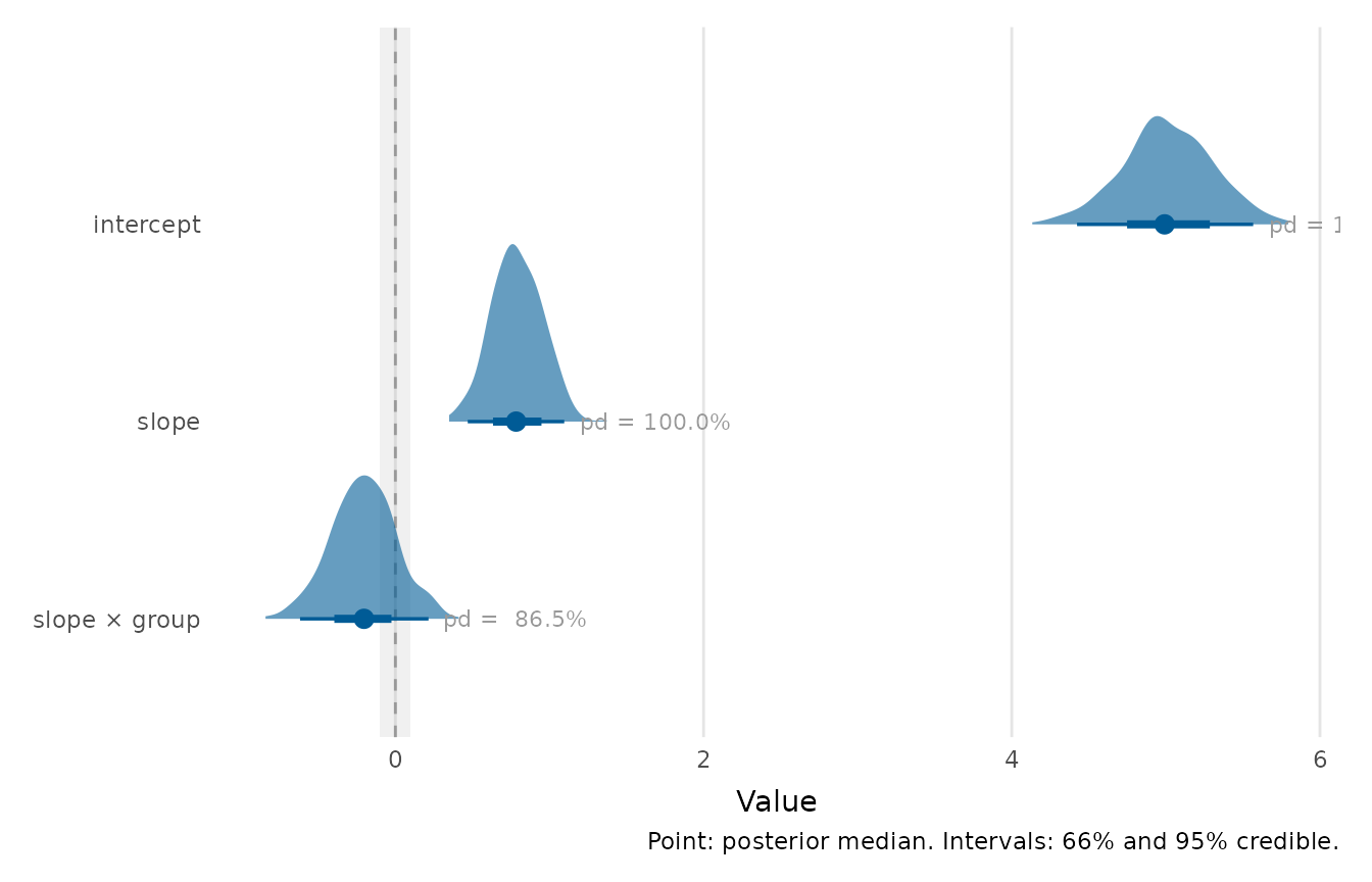
rope: Optional length-2 numeric c(lo, hi) giving a region of practical equivalence to shade behind the distributions.
pd: If TRUE, annotate each parameter with its probability of direction relative to reference_line, the posterior probability that the parameter lies on its majority side of the reference (a value in [0.5, 1]). Requires a finite reference_line.
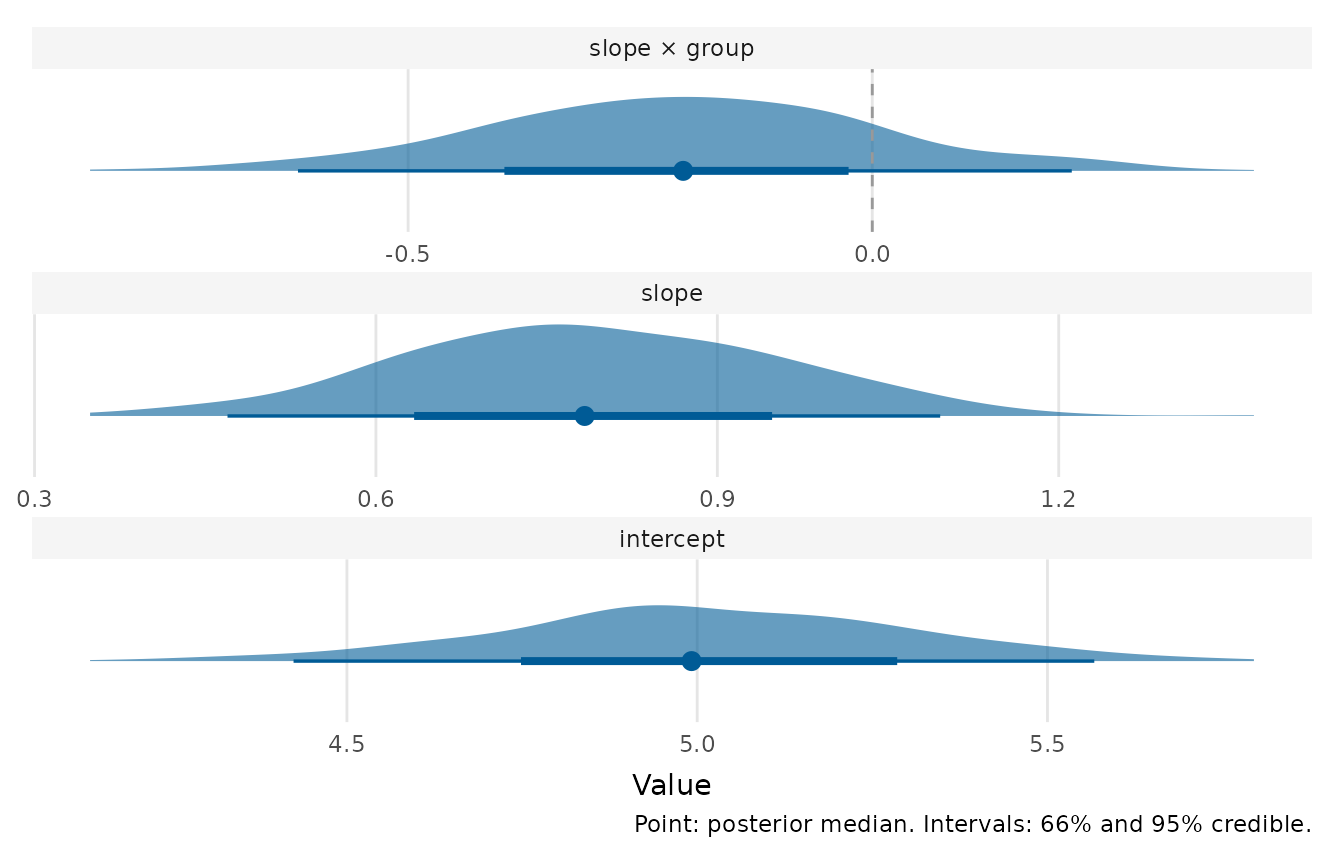
facet: Whether to give each parameter its own panel with a free x-axis, laid out one per row. This keeps the small parameters legible when a large one (typically the intercept) would otherwise stretch the shared axis and squish the rest. Defaults to FALSE. A convenience alias for scales = "free".
scales: Either "fixed" (the default, a single shared x-axis) or "free" (one free-scaled panel per parameter). When facet = TRUE this is forced to "free".
colour, fill: Colours for the point/interval and for the density slab. Default to the depictr brand blue.
rope_fill, rope_alpha: Fill colour and opacity of the ROPE band.
title, x_lab: Plot title and value-axis label.
caption: Plot caption. The default (NULL) auto-captions the interval mass; pass NA to omit a caption.

Value

A ggplot2::ggplot object.

Details

Draws may be supplied in many shapes: a fitted Bayesian model (brms or rstanarm), a posterior draws object, a wide data frame or matrix with one column of draws per parameter, or a long data frame (a parameter column and a value column). For fitted models only the fixed-effect (population) parameters are kept, with the brms b_ prefix stripped.

The slab styles use the 'ggdist' package. When 'ggdist' is not installed the function falls back to the point-and-nested-interval display (equivalent to style = "interval") and emits an informative message.

Examples

# Wide draws: one column per parameter
set.seed(1)
draws <- data.frame(
  intercept = rnorm(400, 5, 0.3),
  slope = rnorm(400, 0.8, 0.15),
  `slope:group` = rnorm(400, -0.2, 0.2),
  check.names = FALSE
)
posterior_plot(draws)

# \donttest{
# A region of practical equivalence and a probability-of-direction label
posterior_plot(draws, rope = c(-0.1, 0.1), pd = TRUE)


# When one parameter dwarfs the others, give each its own free-scaled panel:
posterior_plot(draws, facet = TRUE)

# }