Power and design analysis

library(pilotr)

Simulation-based power addresses how often an analysis would detect an effect if the world matched the specification exactly. pilotr estimates this by repeatedly simulating from the ground-truth specification, fitting the analysis model and recording the proportion of significant results. Beyond power, it reports the design-analysis quantities of Gelman and Carlin (2014), namely the Type S (sign) error and the Type M (magnitude, or exaggeration) ratio.

The mixed-effects examples below use small n_sims, and their results were precomputed with exactly the code shown and shipped with the package, so that the vignette builds quickly. For real planning, we recommend n_sims >= 200, with more replicates for stable Type S and Type M estimates.

Two-group Gaussian

The classic case has a closed-form analytic power, which the simulation matches.

spec <- build_spec(list(
  name = "two_group", seed = 1, design_kind = "between", n_subject = 64,
  factor_name = "group", lev1 = "control", lev2 = "treatment",
  intercept = 100, effect = 5, family = "gaussian",
  resp_name = "score", sigma = 10))

pw <- power_design(spec, n_sims = 500)
unlist(pw[c("power", "type_s", "type_m", "true_effect", "mean_estimate")])

        power        type_s        type_m   true_effect mean_estimate 
     0.504000      0.000000      1.402398      5.000000      4.987050

At roughly 50% power, the Type M ratio is well above 1. Conditional on significance, the estimated effect is exaggerated, even though the average estimate over all replicates is unbiased. This reflects the statistical-significance filter, which is precisely what design analysis is meant to expose.

Crossed mixed-effects designs

A feature that distinguishes pilotr from a marginal simulator is power estimation for crossed by-subject and by-item designs. The R interface fits the maximal model y ~ cond + (1 + cond | subject) + (1 + cond | item) with lme4/lmerTest and tests the fixed effect with Satterthwaite degrees of freedom.

spec_c <- build_spec(list(
  name = "priming", seed = 1, design_kind = "within", include_items = TRUE,
  n_subject = 24, n_item = 18,
  factor_name = "condition", lev1 = "related", lev2 = "unrelated",
  intercept = 6, effect = 0.06,
  subj_int_sd = 0.12, subj_slope_sd = 0.04, subj_corr = 0.2,
  item_int_sd = 0.08, item_slope_sd = 0.02, item_corr = -0.1,
  family = "shifted_lognormal", resp_name = "RT", sigma = 0.3, shift = 200))

# A tiny replicate count keeps the vignette fast. Use 200 or more for real planning.
pm <- power_mixed(spec_c, n_sims = 20)
unlist(pm[c("power", "type_s", "type_m", "n_converged")])

      power      type_s      type_m n_converged 
   0.800000    0.000000    1.193659   20.000000

n_converged reports how many replicates the maximal model actually fit. This is a useful diagnostic in its own right, since convergence problems are common in small crossed designs, and it is the denominator of power, which is the significant proportion among the converged replicates.

power_mixed() carries its own simulation loop over the portable specification, with no other power package underneath it. It covers territory pioneered by simr (Green and MacLeod, 2016) and mixedpower (Kumle, Vo and Draschkow, 2021). pilotr differs in being driven by the cross-language specification, in reporting Type S and Type M errors alongside power and in built-in parallelisation.

A power curve

The following sweep over the number of subjects reports power at each size.

curve <- power_curve_mixed(
  spec_c,
  subject_ns = c(8, 12, 16, 24, 32, 44, 56),
  n_sims = 50)
curve

  n_subject power   type_m n_converged
1         8  0.16 1.998682          50
2        12  0.34 1.639186          50
3        16  0.48 1.404611          50
4        24  0.80 1.189207          50
5        32  0.86 1.129062          50
6        44  0.96 1.046713          50
7        56  0.96 1.048449          50

The sample size the curve implies

The curve is a means to an end. What the analysis is run for is the sample size at which power reaches the target, and that is the number a preregistration quotes. Reading it off the table or the plot judges points whose Monte Carlo intervals overlap, and yields a bare figure with no interval attached to it. target_n() fits the curve and inverts the fit, so the crossing is estimated, and arrives with the uncertainty a simulated curve carries.

solved <- target_n(curve, target = 0.8)
unlist(solved[c("n", "n_lo", "n_hi")])

   n n_lo n_hi 
  29   25   33

Fifty replicates per point is few, and the interval says so. The fit is a binomial regression of power on the square root of the sample size, weighted by the replicates behind each point, and the interval is the delta-method interval that MASS::dose.p() computes for a fitted glm. Nothing is extrapolated: a curve that never reaches the target within the sizes swept is refused, and the refusal reports the range the sweep did cover.

For a curve swept over something other than sample size, solve_curve() is the general form, with transform = "identity" where the axis is an effect size.

Plotting the curve and the solved size together shows what the solve has done.

# The transparent device canvas is what lets the page colour through. A ggplot
# theme alone cannot do it, since the device paints white underneath. The
# website's dark mode then inverts the figure's ink, so the axes and labels
# follow the theme and the figure carries no opaque matte.
library(ggplot2)
# Each power estimate is a proportion over the converged replicates, so it
# carries a binomial Monte Carlo standard error. The shaded band is the 95%
# interval.
curve$se <- sqrt(curve$power * (1 - curve$power) / curve$n_converged)
ggplot(curve, aes(n_subject, power)) +
  geom_hline(yintercept = 0.8, linetype = 2, colour = "grey60") +
  # The solved sample size and its interval. The dashed horizontal line marks
  # the target and the band marks where the curve reaches it.
  annotate("rect", xmin = solved$lo, xmax = solved$hi, ymin = -Inf, ymax = Inf,
           fill = "grey60", alpha = .15) +
  geom_vline(xintercept = solved$value, linetype = 2, colour = "grey60") +
  geom_ribbon(aes(ymin = pmax(0, power - 1.96 * se),
                  ymax = pmin(1, power + 1.96 * se)),
              alpha = .15, fill = "#2C6FB0") +
  geom_line(colour = "#2C6FB0", linewidth = 0.8) +
  geom_point(colour = "#2C6FB0", size = 2.6) +
  scale_y_continuous(limits = c(0, 1)) +
  labs(x = expression(italic(N) ~ "subjects"), y = "Power") +
  theme_minimal(base_size = 12) +
  # theme_minimal still paints a white plot.background over the transparent
  # canvas, so both surfaces have to be cleared for the page colour to reach the
  # figure. The ink is left at its default, because the website inverts the
  # figure in dark mode, which turns the dark axis text light, whereas a fixed
  # mid-grey would be inverted into a muddy tan.
  theme(plot.background  = element_rect(fill = NA, colour = NA),
        panel.background = element_rect(fill = NA, colour = NA),
        panel.grid       = element_line(colour = "grey80"))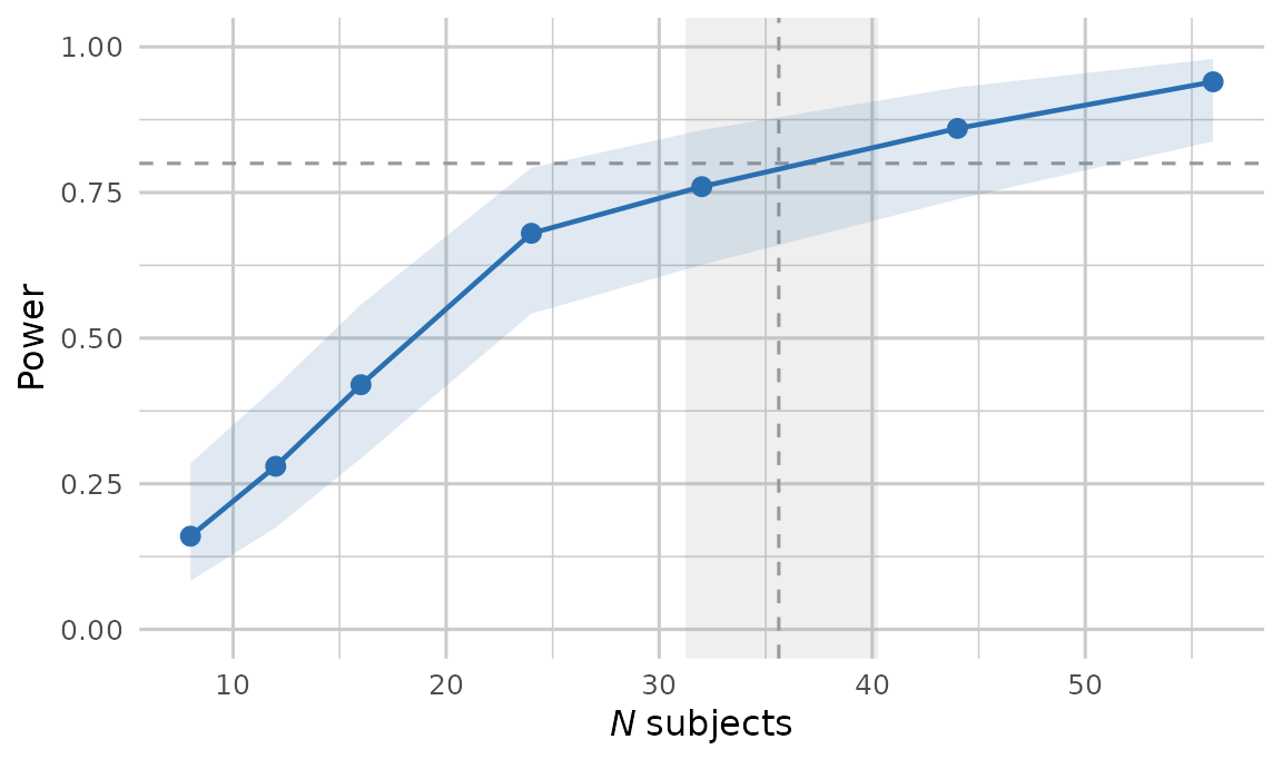

The shaded horizontal band along the curve is the Monte Carlo interval, the binomial standard error of each power estimate over its converged replicates widened to a 95% envelope. The vertical band is the solved sample size and its own interval, which is what the dashed target line invites the reader to guess at.

Parallel execution

Every power and precision analysis in pilotr takes a workers argument that spreads the Monte Carlo replicates across local cores. Each replicate takes its own seed from replicate_seeds(), so the results are identical to a serial run whatever the worker count, and parallelisation costs nothing in reproducibility. The mixed-model fits dominate the running time, which makes the speed-up close to linear in the number of cores. In a sweep the worker pool is created once and reused across all sample sizes.

power_curve_mixed(
  spec_c, subject_ns = seq(20, 60, 10), n_sims = 500, workers = 8)

This design answers a serial bottleneck familiar from simr::powerCurve(), which this package’s maintainer previously worked around by splitting the sample-size grid across separate jobs by hand and recombining the results afterwards (Bernabeu, 2021). In pilotr the same gain takes one argument.

A bridge to the Bayesian workflow

For a confirmatory Bayesian fit, brms_bridge() emits a ready-to-run brms model. It provides the family, the fixed and random-effects formula, and a weakly-informative prior set, all derived from the same specification, so that the planning model and the confirmatory model remain consistent.

brms_bridge(spec_c)

library(brms)
fit <- brm(
  RT ~ effect + (1 + effect | subject) + (1 + effect | item),
  data   = your_data,
  family = shifted_lognormal(),
  prior  = c(
    prior(normal(0, 2.5), class = "Intercept"),
    prior(normal(0, 0.5), class = "b", coef = "effect"),
    prior(normal(0, 1), class = "sd"),
    prior(lkj(2), class = "cor")
  ),
  chains = 4, iter = 4000, warmup = 2000, cores = 4,
  control = list(adapt_delta = 0.95)
)