Parallelizing simr::powercurve() in R
The powercurve function from the R package ‘simr’ (Green & MacLeod, 2016) can incur very long running times when the method used for the calculation of p values is Kenward-Roger or Satterthwaite (see Luke, 2017). Here I suggest three ways for cutting down this time.
Where possible, use a high-performance (or high-end) computing cluster. This removes the need to use personal computers for these long jobs.
In case you’re using the
fixed()parameter of thepowercurvefunction, and calculating the power for different effects, run these at the same time (‘in parallel’) on different machines, rather than one after another.Parallelize the
breaksargument. Thebreaksargument of thepowercurvefunction allows the calculation of power for different levels of the grouping factor passed toalong. Some grouping factors are participant, trial and item. Thebreaksargument sets the different sample sizes for which power will be calculated. Parallelizingbreaksis done by running each number of levels in a separate function. When each has been run and saved, they arecombined to allow the plotting. This procedure is demonstrated below.
Parallelizing breaks
Let’s do a minimal example using a toy lmer model. A power curve will be created for the fixed effect of x along different sample sizes of the grouping factor g.
Notice that the six sections of the power curve below are serially arranged, one after another. In contrast, to enable parallel processing, each power curve would be placed in a single script, and they would all be run at the same time.
Although the power curves below run in a few minutes, the settings that are often used (e.g., a larger model; fixed('x', 'sa') instead of fixed('x'); nsim = 500 instead of nsim = 50) take far longer. That is where parallel processing becomes useful.1
library(lme4)
library(simr)

# Toy model with data from 'simr' package
fm = lmer(y ~ x + (x | g), data = simdata)

# Extend sample size of `g`
fm_extended_g = extend(fm, along = 'g', n = 12)

# Parallelize `breaks` by running each number of levels in a separate function.

# 4 levels of g
pwcurve_4g = powerCurve(fm_extended_g, fixed('x'), along = 'g', breaks = 4,
                        nsim = 50, seed = 123,
                        # No progress bar
                        progress = FALSE)

# 6 levels of g
pwcurve_6g = powerCurve(fm_extended_g, fixed('x'), along = 'g', breaks = 6,
                        nsim = 50, seed = 123,
                        # No progress bar
                        progress = FALSE)

# 8 levels of g
pwcurve_8g = powerCurve(fm_extended_g, fixed('x'), along = 'g', breaks = 8,
                        nsim = 50, seed = 123,
                        # No progress bar
                        progress = FALSE)

# 10 levels of g
pwcurve_10g = powerCurve(fm_extended_g, fixed('x'), along = 'g', breaks = 10,
                        nsim = 50, seed = 123,
                        # No progress bar
                        progress = FALSE)

# 12 levels of g
pwcurve_12g = powerCurve(fm_extended_g, fixed('x'), along = 'g', breaks = 12,
                        nsim = 50, seed = 123,
                        # No progress bar
                        progress = FALSE)
Having saved each section of the power curve, we must now combine them to be able to plot them together (if you wish to automatise this procedure, consider this function).
# Create a destination object using any of the power curves above.
all_pwcurve = pwcurve_4g

# Combine results
all_pwcurve$ps = c(pwcurve_4g$ps[1], pwcurve_6g$ps[1], pwcurve_8g$ps[1],
                   pwcurve_10g$ps[1], pwcurve_12g$ps[1])

# Combine the different numbers of levels.
all_pwcurve$xval = c(pwcurve_4g$nlevels, pwcurve_6g$nlevels, pwcurve_8g$nlevels,
                     pwcurve_10g$nlevels, pwcurve_12g$nlevels)

print(all_pwcurve)
## Power for predictor 'x', (95% confidence interval),
## by number of levels in g:
## 4: 46.00% (31.81, 60.68) - 40 rows
## 6: 74.00% (59.66, 85.37) - 60 rows
## 8: 92.00% (80.77, 97.78) - 80 rows
## 10: 98.00% (89.35, 99.95) - 100 rows
## 12: 100.0% (92.89, 100.0) - 120 rows
##
## Time elapsed: 0 h 0 m 7 splot(all_pwcurve, xlab = 'Levels of g')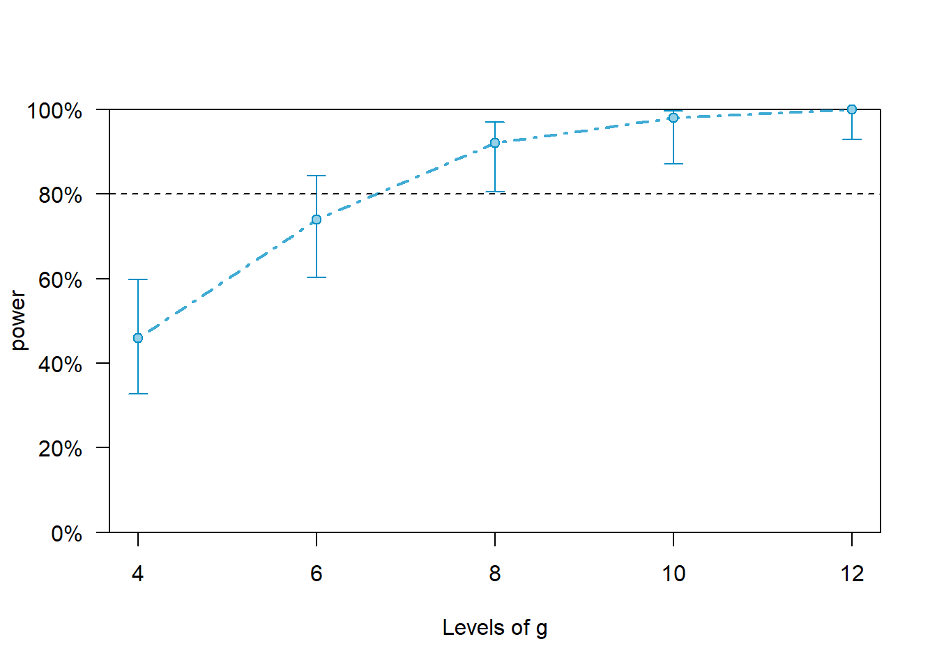
# For reproducibility purposes
sessionInfo()
## R version 4.5.1 (2025-06-13 ucrt)
## Platform: x86_64-w64-mingw32/x64
## Running under: Windows 11 x64 (build 26200)
##
## Matrix products: default
## LAPACK version 3.12.1
##
## locale:
## [1] LC_COLLATE=English_United Kingdom.utf8
## [2] LC_CTYPE=English_United Kingdom.utf8
## [3] LC_MONETARY=English_United Kingdom.utf8
## [4] LC_NUMERIC=C
## [5] LC_TIME=English_United Kingdom.utf8
##
## time zone: Europe/London
## tzcode source: internal
##
## attached base packages:
## [1] stats graphics grDevices datasets utils methods base
##
## other attached packages:
## [1] simr_1.0.7 lme4_1.1-37 Matrix_1.7-3
## [4] knitr_1.50 xaringanExtra_0.8.0
##
## loaded via a namespace (and not attached):
## [1] tidyr_1.3.1 sass_0.4.10 generics_0.1.4 renv_1.1.5
## [5] stringi_1.8.7 blogdown_1.21 lattice_0.22-7 digest_0.6.37
## [9] magrittr_2.0.3 evaluate_1.0.4 grid_4.5.1 bookdown_0.43
## [13] iterators_1.0.14 fastmap_1.2.0 plyr_1.8.9 jsonlite_2.0.0
## [17] backports_1.5.0 Formula_1.2-5 mgcv_1.9-3 purrr_1.1.0
## [21] jquerylib_0.1.4 abind_1.4-8 reformulas_0.4.1 Rdpack_2.6.4
## [25] cli_3.6.5 rlang_1.1.6 rbibutils_2.3 binom_1.1-1.1
## [29] splines_4.5.1 plotrix_3.8-4 cachem_1.1.0 yaml_2.3.10
## [33] RLRsim_3.1-8 parallel_4.5.1 tools_4.5.1 pbkrtest_0.5.5
## [37] uuid_1.2-1 nloptr_2.2.1 minqa_1.2.8 dplyr_1.1.4
## [41] boot_1.3-31 broom_1.0.9 vctrs_0.6.5 R6_2.6.1
## [45] lifecycle_1.0.4 stringr_1.5.1 car_3.1-3 MASS_7.3-65
## [49] pkgconfig_2.0.3 bslib_0.9.0 pillar_1.11.0 glue_1.8.0
## [53] Rcpp_1.1.0 tidyselect_1.2.1 tibble_3.3.0 xfun_0.52
## [57] htmltools_0.5.8.1 nlme_3.1-168 rmarkdown_2.29 carData_3.0-5
## [61] compiler_4.5.1Just the code
library(lme4)
library(simr)

# Toy model
fm = lmer(y ~ x + (x | g), data = simdata)

# Extend sample size of `g`
fm_extended_g = extend(fm, along = 'g', n = 12)

# Parallelize `breaks` by running each number of levels in a separate function.

# 4 levels of g
pwcurve_4g = powerCurve(fm_extended_g, fixed('x'), along = 'g', breaks = 4,
                        nsim = 50, seed = 123,
                        # No progress bar
                        progress = FALSE)

# 6 levels of g
pwcurve_6g = powerCurve(fm_extended_g, fixed('x'), along = 'g', breaks = 6,
                        nsim = 50, seed = 123,
                        # No progress bar
                        progress = FALSE)

# 8 levels of g
pwcurve_8g = powerCurve(fm_extended_g, fixed('x'), along = 'g', breaks = 8,
                        nsim = 50, seed = 123,
                        # No progress bar
                        progress = FALSE)

# 10 levels of g
pwcurve_10g = powerCurve(fm_extended_g, fixed('x'), along = 'g', breaks = 10,
                        nsim = 50, seed = 123,
                        # No progress bar
                        progress = FALSE)

# 12 levels of g
pwcurve_12g = powerCurve(fm_extended_g, fixed('x'), along = 'g', breaks = 12,
                        nsim = 50, seed = 123,
                        # No progress bar
                        progress = FALSE)


# Create a destination object using any of the power curves above.
all_pwcurve = pwcurve_4g

# Combine results
all_pwcurve$ps = c(pwcurve_4g$ps[1], pwcurve_6g$ps[1], pwcurve_8g$ps[1],
                   pwcurve_10g$ps[1], pwcurve_12g$ps[1])

# Combine the different numbers of levels.
all_pwcurve$xval = c(pwcurve_4g$nlevels, pwcurve_6g$nlevels, pwcurve_8g$nlevels,
                     pwcurve_10g$nlevels, pwcurve_12g$nlevels)


print(all_pwcurve)

plot(all_pwcurve, xlab = 'Levels of g')
References
Brysbaert, M., & Stevens, M. (2018). Power analysis and effect size in mixed effects models: A tutorial. Journal of Cognition, 1(1), 9. http://doi.org/10.5334/joc.10
Green, P., & MacLeod, C. J. (2016). SIMR: An R package for power analysis of generalized linear mixed models by simulation. Methods in Ecology and Evolution 7(4), 493–498, https://doi.org/10.1111/2041-210X.12504
Kumle, L., Vo, M. L. H., & Draschkow, D. (2021). Estimating power in (generalized) linear mixed models: An open introduction and tutorial in R. Behavior Research Methods, 1–16. https://doi.org/10.3758/s13428-021-01546-0
Luke, S. G. (2017). Evaluating significance in linear mixed-effects models in R. Behavior Research Methods, 49(4), 1494–1502. https://doi.org/10.3758/s13428-016-0809-y
The number of simulations set by
nsimshould be larger (Brysbaert & Stevens, 2018; Green & MacLeod, 2016). In addition, the effect size forxshould be adjusted to the value that best fits with the planned study (Kumle et al., 2021).↩︎