
When sample sizes are large, or when the question of interest is whether an effect is practically meaningful, power against a point null is often the wrong target. pilotr implements a precision-based design analysis against a region of practical equivalence (ROPE). This is a fast, frequentist analogue of the Bayesian approach that compares a highest-density interval with a ROPE.
As in the power vignette, the fixed-N analysis below uses a small
n_simsso that the vignette builds quickly, and the sample-size sweep, which needs far more model fits, was precomputed with exactly the code shown and shipped with the package. For real planning we recommendn_sims >= 200, the value the sweep uses.
The idea
Over Monte Carlo replicates, and for each focal fixed effect, pilotr records the 95% confidence interval and whether it falls determinately outside the ROPE (the effect is practically meaningful) or entirely inside it (practical equivalence to zero), together with the expected interval width. The interval is a Wald approximation, the estimate plus or minus 1.96 standard errors, chosen for speed and for comparability across replicates. Sweeping sample size then locates the minimum N at which a focal effect reaches a determinate decision with a target probability.
A worked design
We reuse the crossed priming design, which represents a small priming
effect on log reaction time. Every subject sees every item in both
conditions. A counterbalanced study, in which each subject sees each
item in one condition only, has half the observations and wider
intervals, so it needs more subjects than the sweep below finds. Plan
such a study with counterbalance = TRUE in
build_spec(), which needs specification version 0.4, or
with the two-list encoding among the worked
encodings of the specification, which earlier releases read too.
spec_c <- build_spec(list(
  name = "priming", seed = 1, design_kind = "within", include_items = TRUE,
  n_subject = 24, n_item = 18,
  factor_name = "condition", lev1 = "related", lev2 = "unrelated",
  intercept = 6, effect = 0.05,
  subj_int_sd = 0.12, subj_slope_sd = 0.04, subj_corr = 0.2,
  item_int_sd = 0.08, item_slope_sd = 0.02, item_corr = -0.1,
  family = "shifted_lognormal", resp_name = "RT", sigma = 0.3, shift = 200))
So that the analysis can run from the specification alone, pilotr auto-derives the analysis model, including the contrast columns, the response transform and the mixed-model formula.
model_formula(spec_c).y ~ effect + (1 + effect | subject) + (1 + effect | item)The companion model_data() adds the other two
derivations to a simulated data set, the numeric effect
contrast column the formula’s terms refer to and the .y
response, here the log-transformed RT because the family is
shifted_lognormal.
head(model_data(spec_c, simulate_design(spec_c))) subject item condition RT .y effect
1 1 1 related 688.7993 6.191952 -0.5
2 1 1 unrelated 778.3731 6.360219 0.5
3 1 2 related 884.1392 6.528161 -0.5
4 1 2 unrelated 788.8995 6.378256 0.5
5 1 3 related 651.0253 6.111523 -0.5
6 1 3 unrelated 518.3355 5.763106 0.5Precision at a fixed N
We declare the focal effect (its coefficient name and true value) and a ROPE half-width. Here the effect lives on the log scale, and we treat anything smaller than 0.02 as practically equivalent to zero.
pr <- precision_design(
  spec_c, focal = c(effect = 0.05), rope = 0.02, n_sims = 25)
pr
param true mean_ci_width p_meaningful p_meaningful_mcse p_meaningful_lo
1 effect 0.05 0.09809118 0.28 0.08979978 0.1428385
p_meaningful_hi p_equivalent p_equivalent_mcse p_equivalent_lo
1 0.4757661 0 0 0
p_equivalent_hi n_attempted n_returned n_converged n_singular n_warning
1 0.1331923 25 25 8 17 0
fitter
1 lme4::lmer, Wald zThe columns are interpreted as follows. p_meaningful is
the probability the 95% CI lands entirely outside the ROPE, a
determinate ‘meaningful’ decision. p_equivalent is the
probability it lands entirely inside, a determinate ‘equivalent’
decision. mean_ci_width is the expected precision.
Sweeping sample size
The same ROPE has to be carried into the sweep. Leaving
rope at its default would compare the interval against a
region as wide as the effect itself, and the decision probability would
then fall away as N grew, which is backwards.
prc <- precision_curve(spec_c, focal = c(effect = 0.05),
                       subject_ns = c(15, 30, 60, 100, 140, 180, 220, 260),
                       rope = 0.02, n_sims = 200)
print(prc[, c("n_subject", "p_meaningful", "p_equivalent", "mean_ci_width",
              "n_returned", "n_singular")], digits = 3)
n_subject p_meaningful p_equivalent mean_ci_width n_returned n_singular
1 15 0.140 0 0.1215 200 156
2 30 0.300 0 0.0834 200 141
3 60 0.550 0 0.0605 200 113
4 100 0.680 0 0.0478 200 97
5 140 0.870 0 0.0407 200 82
6 180 0.885 0 0.0370 200 74
7 220 0.945 0 0.0339 200 46
8 260 0.945 0 0.0322 200 55As N grows the interval tightens and
p_meaningful rises, so the design reaches a determinate
decision more reliably. That is a more informative criterion than power
against a point null, because it asks whether the study can distinguish
the effect from a negligible one, where power asks only whether it can
be distinguished from zero. Each probability is a proportion over the
replicates that returned an estimate, n_returned, 200 at
each size here, so its Monte Carlo standard error is at most 0.035. The
figure below draws the Wilson interval of p_meaningful as a
band.
n_singular counts the fits whose variance estimates sat
on a boundary, 156 at 15 subjects and 55 at 260.
n_converged, in the full result, counts those with neither
a singular fit nor a warning. Singular fits are kept in the proportions,
since their fixed-effect estimates remain interpretable and discarding
them would bias the result. A large n_singular says that
the model is richer than the design can support at that size.
Scanning the table for the smallest simulated N that meets a
target of ‘p_meaningful ≥ 0.90’ gives 220 subjects. That
answer is a property of where the grid points happen to fall, and it
comes without an interval. solve_curve() fits the decision
probability against the sample size and inverts the fit, so all eight
points inform the answer, where scanning the table uses only the two
either side of the target.
solved <- solve_curve(prc, target = 0.9)
unlist(solved[c("value", "lo", "hi", "dispersion")])
value lo hi dispersion
181.127671 161.378958 202.016032 2.287547 The fitted crossing is 181 subjects. With 200 replicates per point,
this design needs somewhere between 161 and 203 subjects to reach a
determinate ROPE decision nine times in ten. The 220 read by eye lies
above that interval. Only the interval says how far the answer could
move, and a preregistration quoting a single figure would be claiming
more than the simulation supports. The fit is a binomial probit
regression weighted by the replicates behind each point, and the
interval is the delta-method interval that MASS::dose.p()
computes for a fitted glm.
The dispersion is Pearson’s chi-square over its degrees
of freedom, floored at 1, and here it is 2.29. Above 1, it says the
points scatter about the fitted curve more than their replicate counts
alone would explain, and the interval is widened to match. That is the
heterogeneity factor of classical probit analysis. Nothing is
extrapolated either: a curve that never reaches the target within the
sizes swept is refused, and the refusal reports the range the sweep did
cover.
power_report() turns the solve into the sample-size
justification a preregistration needs. It takes a
precision_design() result at the chosen size, the
target_n() result for this curve, which rounds the solve up
to whole subjects, and the region of practical equivalence as
rope. It writes each effect’s mean interval width and the
probabilities of the two decisions, each with its Monte Carlo error,
beside the solved size and its interval. The power vignette writes one for a power
analysis.
p_equivalent stays at 0 throughout, and correctly so.
The true effect of 0.05 lies outside the ROPE by construction, so no
interval should ever land entirely inside it. The column earns its place
in designs where practical equivalence is the hypothesis of
interest.
library(ggplot2)
# Each probability is a proportion over the replicates that returned an
# estimate, and the sweep carries its 95% Wilson interval, which the band draws.
# The two panels are on different scales, hence the free y axis.
panels <- c("P(CI outside the ROPE)", "Mean 95% CI width")
long <- rbind(
  data.frame(n_subject = prc$n_subject, panel = panels[1], y = prc$p_meaningful,
             lo = prc$p_meaningful_lo, hi = prc$p_meaningful_hi),
  data.frame(n_subject = prc$n_subject, panel = panels[2],
             y = prc$mean_ci_width,
             lo = NA, hi = NA))
long$panel <- factor(long$panel, levels = panels)
# 0.90 is the target decision probability. 0.06 is the width at which a CI
# centred on the true effect just clears the ROPE, that is 2 * (0.05 - 0.02).
refs <- data.frame(panel = factor(panels, levels = panels), ref = c(0.90, 0.06))
# The solved sample size and its interval, drawn only on the decision panel,
# since the width panel is on a different scale and answers a different question.
solve_band <- data.frame(panel = factor(panels[1], levels = panels),
                         lo = solved$lo, hi = solved$hi, at = solved$value)

ggplot(long, aes(n_subject, y)) +
  geom_hline(data = refs, aes(yintercept = ref), linetype = 2,
             colour = "grey60") +
  geom_rect(data = solve_band, inherit.aes = FALSE,
            aes(xmin = lo, xmax = hi, ymin = -Inf, ymax = Inf),
            fill = "grey60", alpha = .15) +
  geom_vline(data = solve_band, aes(xintercept = at), linetype = 2,
             colour = "grey60") +
  geom_ribbon(aes(ymin = lo, ymax = hi), alpha = .15, fill = "#2C6FB0",
              na.rm = TRUE) +
  geom_line(colour = "#2C6FB0", linewidth = 0.8) +
  geom_point(colour = "#2C6FB0", size = 2.2) +
  facet_wrap(~ panel, scales = "free_y") +
  labs(x = expression(italic(N) ~ "subjects"), y = NULL) +
  theme_minimal(base_size = 12) +
  # theme_minimal still paints a white plot.background over the transparent
  # canvas, so both surfaces have to be cleared for the page colour to reach the
  # figure.
  theme(plot.background  = element_rect(fill = NA, colour = NA),
        panel.background = element_rect(fill = NA, colour = NA),
        panel.grid       = element_line(colour = "grey80"),
        strip.background = element_rect(fill = NA, colour = NA))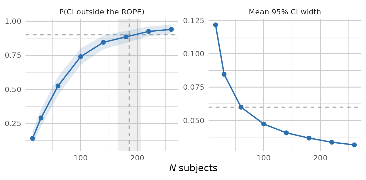
The two panels answer the same question from either side. On the left, the horizontal dashed line marks the 0.90 target, and the vertical band the sample size solved against it. On the right the dashed line marks a width of 0.06, which is where a confidence interval centred on the true effect just clears a ROPE of 0.02, since the interval has to keep its lower limit above the ROPE and so must be narrower than 2 × (0.05 − 0.02). Width falls below that line well before the decision probability reaches 0.90, because an interval centred exactly on the true effect is the best case and sampling variation moves the centre about.
See also
The power vignette covers simulation-based power and Type S/M errors. The getting-started vignette covers the core simulate-and-inspect loop.