
Behavioural outcomes are seldom Gaussian. pilotr maps the linear predictor to an outcome through one of eight response families. An important consequence is that the fixed intercept and effect live on the family’s own scale. That scale is the identity for the Gaussian and ex-Gaussian families, the log scale for lognormal reaction times, reading times and counts, and the logit scale for accuracy, ordinal and proportion outcomes. This vignette presents each family with scale-appropriate parameters.
The helper below builds a two-group between-subjects design and reports the group means.
demo <- function(family, intercept, effect, n = 4000, ...) {
  spec <- build_spec(list(
    name = family, seed = 1, design_kind = "between", n_subject = n,
    factor_name = "group", lev1 = "control", lev2 = "treatment",
    intercept = intercept, effect = effect, family = family,
    resp_name = "", ...))
  d <- simulate_design(spec)
  y <- d[[spec$response$name]]
  list(spec = spec, data = d, y = y, by_group = tapply(y, d$group, mean))
}

library(ggplot2)
fam_hist <- function(y, fill, title, xlab) {
  ggplot(data.frame(y = y), aes(y)) +
    geom_histogram(bins = 40, fill = fill, colour = NA) +
    labs(title = title, x = xlab, y = "count") +
    theme_minimal(base_size = 12) +
    # theme_minimal still paints a white plot.background over the transparent
    # device canvas, so both surfaces have to be cleared for the page colour to
    # reach the figure. The ink stays at its default, because the website
    # inverts the figure in dark mode, which turns the dark axis text light of
    # its own accord.
    theme(plot.background  = element_rect(fill = NA, colour = NA),
          panel.background = element_rect(fill = NA, colour = NA),
          panel.grid       = element_line(colour = "grey80"))
}
Gaussian
This is the default, with
and residual standard deviation sigma. It suits continuous,
roughly symmetric outcomes such as ratings averaged over many trials or
standardised scores.
  control treatment
    97.50    102.41
fam_hist(g$y, "#2C6FB0", "Gaussian", "score")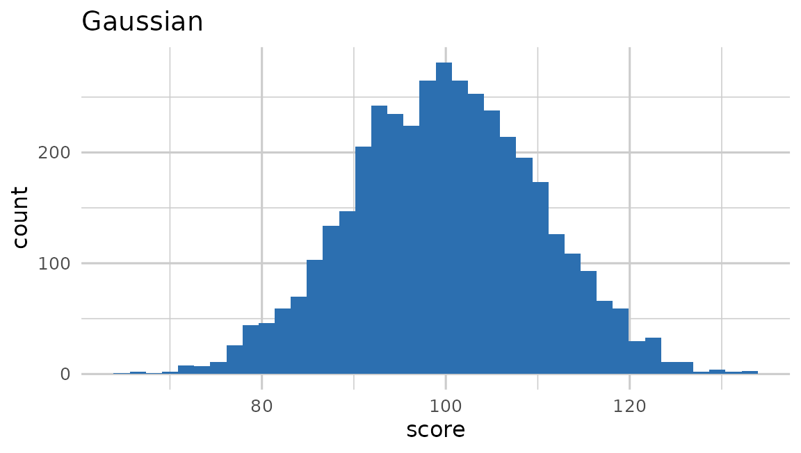
Shifted lognormal (reaction times)
Reaction times are right-skewed and bounded below. pilotr models them
as
,
with the effect on the log scale. An intercept of 6 implies a typical RT
near exp(6) ms above the shift.
rt <- demo(
  "shifted_lognormal", intercept = 6, effect = 0.1, sigma = 0.3, shift = 200
)
round(rt$by_group, 1)
control treatment
600.6 642.6
fam_hist(rt$y, "#B0402C", "Shifted lognormal (RT)", "RT (ms)")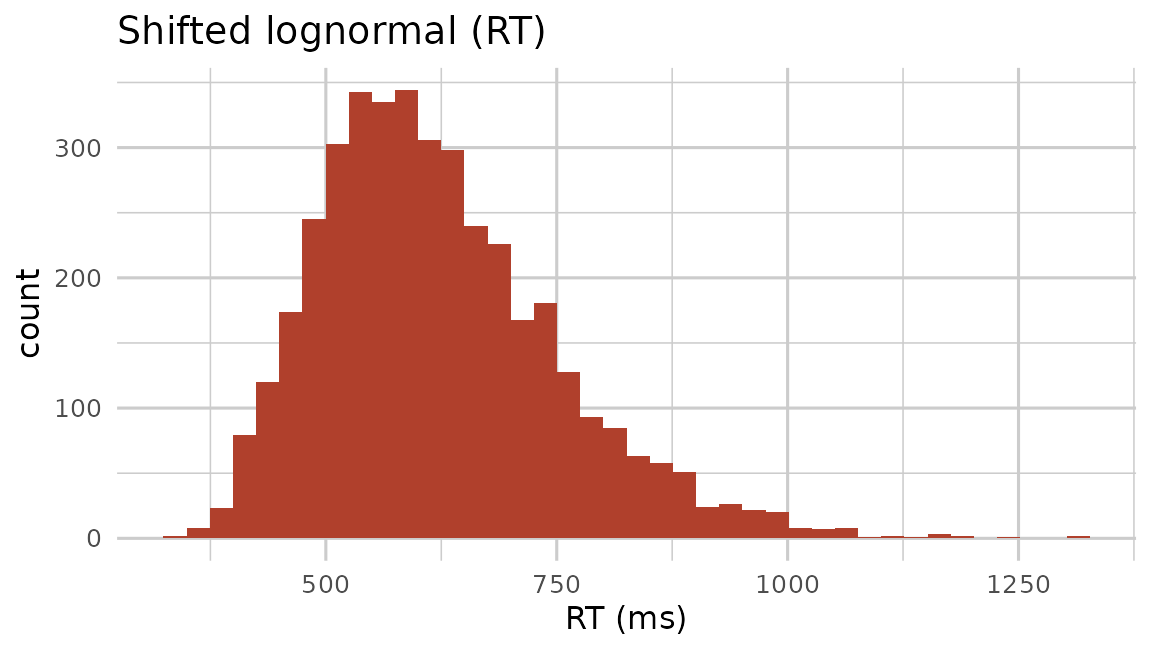
Lognormal (positive continuous)
The plain lognormal family is the shifted lognormal
without the shift,
,
suited to positive continuous outcomes such as per-word reading times.
As with reaction times the effect is on the log scale.
  control treatment
    400.6     442.6
fam_hist(ln$y, "#7A4FB0", "Lognormal", "reading time (ms)")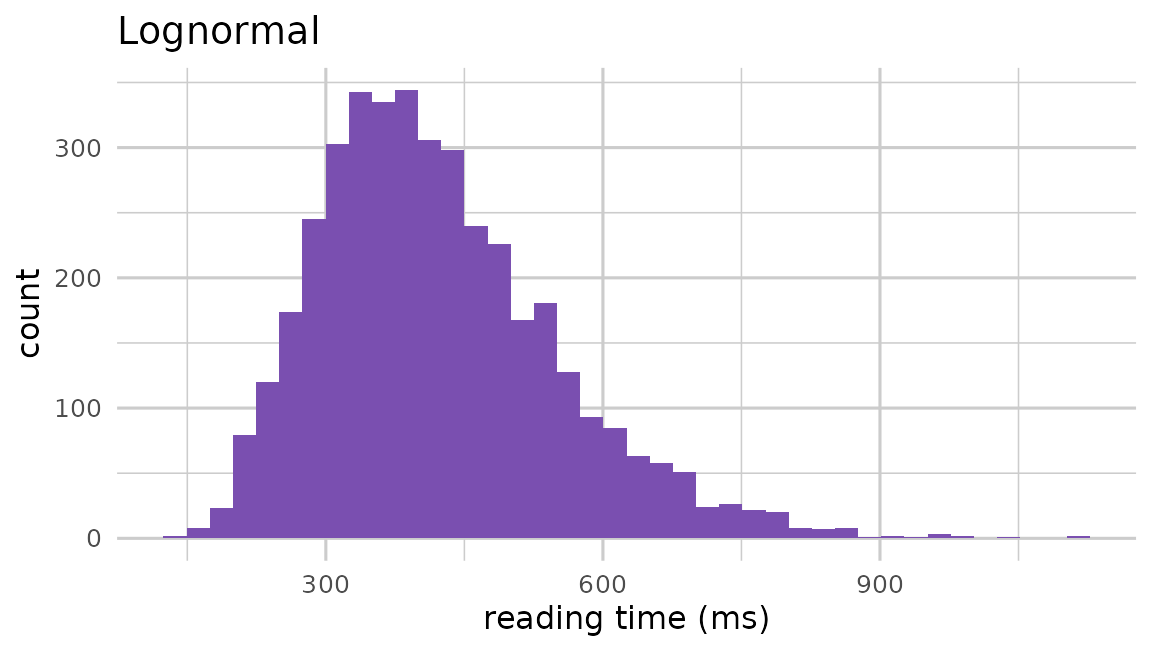
Bernoulli (accuracy)
Binary accuracy is modelled through a logit link. The intercept is the log-odds of a correct response, and the effect is a log-odds difference between conditions.
  control treatment
    0.446     0.569
Poisson (counts)
Counts via a log link (e.g. number of fixations, errors or events).
An intercept of 1.5 implies a base rate near exp(1.5).
  control treatment
     3.85      5.18
table(cts$y)[1:8]
  0   1   2   3   4   5   6   7
 41 225 466 698 711 659 466 334
Ordinal (Likert)
Ordered categorical responses via a cumulative-logit model with user thresholds. The effect shifts the latent distribution across the thresholds.
ord <- build_spec(list(
  name = "likert", seed = 1, design_kind = "between", n_subject = 4000,
  factor_name = "group", lev1 = "control", lev2 = "treatment",
  intercept = 0, effect = 0.8, family = "ordinal", resp_name = "rating",
  thresholds = "-2, -0.6, 0.6, 2"))
r <- simulate_design(ord)
# category proportions by group
round(prop.table(table(r$group, r$rating), 1), 2)
               1    2    3    4    5
  control   0.16 0.30 0.27 0.19 0.08
  treatment 0.09 0.18 0.29 0.28 0.17
Beta (proportions)
Bounded proportions in (0, 1) are modelled through a mean–precision
parameterisation. The mean is logit⁻¹(η) and
phi is the precision, with larger values giving a tighter
distribution.
bt <- demo("beta", intercept = 0, effect = 0.8, phi = 8)
round(bt$by_group, 3)   # mean proportion by group
control treatment
0.400 0.592
fam_hist(bt$y, "#2E8B57", "Beta", "proportion")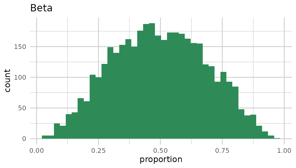
Every simulated proportion lies strictly inside (0, 1), as
brms::Beta() and other Beta regressions require. Near a
ceiling or a floor, a draw can round to exactly 1 or 0 in double
precision, and it then becomes the nearest double inside the interval. A
round set for the family must be at least 1. A value
rounded onto 0 or 1 then becomes the nearest value inside the interval
at that many decimals, 0.001 or 0.999 at three. A linear predictor
beyond about 36.7, or below about −745, leaves a shape parameter of zero
and is refused. When mu * phi or
(1 - mu) * phi is well below 1, many rows sit at the
bounds, and ?brms_bridge explains how they weigh on a Beta
fit.
Choosing a family
The families above, together with the ex-Gaussian, cover the outcome types a behavioural study usually produces. The table below sets each one against the scale its intercept and effect are written on.
| Outcome | Family | Scale of the effect |
|---|---|---|
| Continuous, symmetric | gaussian |
identity |
| Reaction time | shifted_lognormal |
log |
| Positive continuous (e.g. reading time) | lognormal |
log |
| Reaction time, on the response scale | exgaussian |
identity |
| Accuracy (0/1) | bernoulli |
logit |
| Counts | poisson |
log |
| Likert / ordered categories | ordinal |
logit (cumulative) |
| Proportions in (0, 1) | beta |
logit (mean) |
These match the families that researchers fit in lme4,
glmmTMB and brms, so a design simulated here
corresponds to the model that will later be fit. pilotr’s own
power_mixed() and precision_design() fit the
continuous families with lmer() and accuracy and counts
with glmer(), so their estimates are on the scale in the
table’s last column. Ordinal and Beta outcomes have no frequentist model
there yet, and their design analysis runs in brms through
generate_design_analysis(). The point-and-click application
exposes six of the eight families. The full engine, including the plain
lognormal, the ex-Gaussian, continuous predictors, interactions, nesting
and partial crossing, is reached by writing the specification directly,
as the last section of this vignette shows.
The exgaussian family, new in 0.3, takes
sigma and beta and draws a normal plus an
exponential, mean-centred by subtracting the mean of the exponential so
that
remains the mean of the response. That is brms’s
exgaussian(mu, sigma, beta) parameterisation, so a
specification and the model fitted to it agree on what the intercept
means. A shifted lognormal will not stand in for it, because
model_data() logs the response back and leaves a symmetric
residual on the analysis scale. build_spec() does not cover
the family either, so an ex-Gaussian design has to be written out by
hand.
Writing the specification directly
The specification is a plain list, so richer designs than the builder
covers can be assembled by hand. Starting from a
build_spec() result, the example below adds a continuous
item-level predictor, an interaction with the categorical effect, a
per-subject item subset (partial crossing) and an extra grouping factor
that nests subjects.
spec <- build_spec(list(
  name = "reading", seed = 1, design_kind = "within", include_items = TRUE,
  n_subject = 12, n_item = 24,
  factor_name = "condition", lev1 = "related", lev2 = "unrelated",
  intercept = 6, effect = 0.05,
  subj_int_sd = 0.12, subj_slope_sd = 0.04, subj_corr = 0.2,
  item_int_sd = 0.08, item_slope_sd = 0.02, item_corr = -0.1,
  family = "lognormal", resp_name = "RT", sigma = 0.25))

spec$predictors <- list(
  list(name = "freq", varies_by = "item", mean = 0, sd = 1)
)
# an interaction with the effect
spec$fixed$coefficients[["effect:freq"]] <- 0.02
# each subject sees 10 of the 24 items
spec$units$item$per_subject <- 10
# subjects nested in classes
spec$random$class <- list(over = "subject", n = 6, intercept_sd = 0.05)

head(simulate_design(spec))
subject item class condition freq RT
1 1 2 1 related 2.355932 558.9340
2 1 2 1 unrelated 2.355932 609.7181
3 1 7 1 related -2.020596 449.9641
4 1 7 1 unrelated -2.020596 630.8554
5 1 8 1 related 1.017863 507.4829
6 1 8 1 unrelated 1.017863 445.2669The derived columns follow from the specification: freq
is the continuous predictor and class is the nesting
factor. The auto-derived formula picks up the interaction as
effect_freq and the extra grouping factor as
(1 | class).
model_formula(spec).y ~ effect + effect_freq + (1 + effect | subject) + (1 + effect |
item) + (1 | class)Ready-to-run specifications of this kind, including a
continuous-predictor reading-time design, a nested-clusters design and a
partial-crossing design, ship in the repository’s spec/examples/
directory, and load_spec() reads any of them back.