Computes a variance inflation factor for each term in a model and shows
them as a bar chart, with a reference line at the usual rule of thumb
(threshold). High bars flag predictors whose coefficients are unstable
because they are collinear with the others. Values are computed from base R
(no 'car' dependency).
Usage
vif_plot(model, threshold = 5, palette = depictr_palette(2), title = NULL)Arguments
- model
A fitted
lmorglmmodel with at least two predictors.- threshold
Reference value for the ordinary VIF, drawn as a line. For models with multi-column terms it is shown on the \(\mathrm{GVIF}^{1/(2\,\mathrm{df})}\) scale as \(\sqrt{\mathrm{threshold}}\).
- palette
Length-2 colours encoding terms below and above the threshold. Defaults to the colourblind-safe
depictr_palette()pair (blue / orange).- title
Plot title.
Value
A ggplot2::ggplot object.
Details
For single-degree-of-freedom terms this is the ordinary VIF, \(1/(1-R^2)\).
For terms that span several design-matrix columns (multi-level factors, or
spline/polynomial bases) the function reports the generalised VIF of Fox and
Monette (1992): with \(R\) the correlation matrix of the coefficient
estimates other than the intercept, \(R_{11}\) the block for the term and
\(R_{22}\) the block for the remaining coefficients,
$$\mathrm{GVIF} = \frac{\det(R_{11})\,\det(R_{22})}{\det(R)}.$$
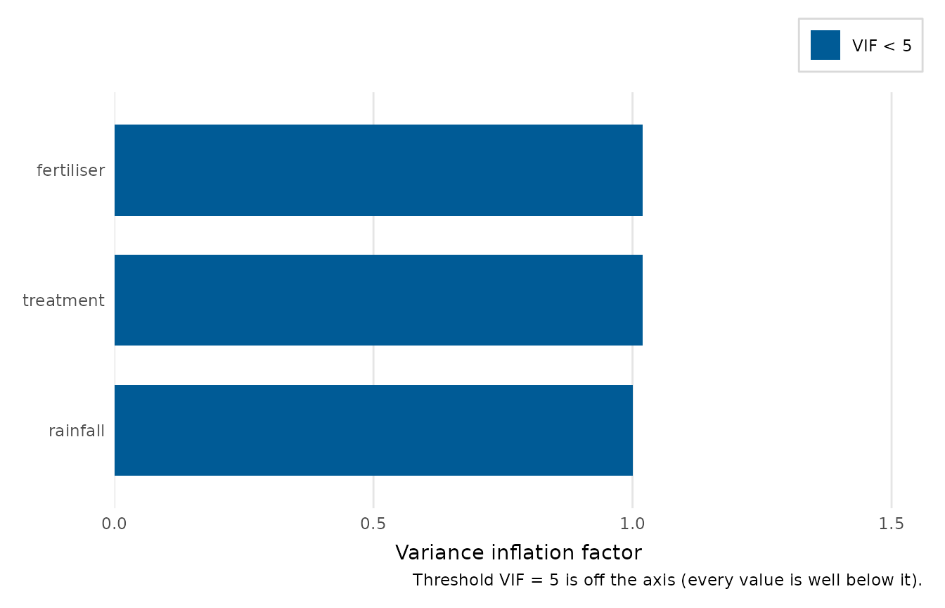
When every term has a single degree of freedom the bars are the ordinary
VIFs, on a plain "Variance inflation factor" axis with the reference line at
threshold. If any term spans several columns the bars switch to the
comparable \(\mathrm{GVIF}^{1/(2\,\mathrm{df})}\) (which for a single-df
term equals \(\sqrt{\mathrm{VIF}}\)) and the reference line moves to
\(\sqrt{\mathrm{threshold}}\) accordingly. The x-axis is kept tight to the
data: when every bar is comfortably below the threshold the line is reported
in the caption rather than drawn into a wide empty band.
The correlations come from the fit's unscaled coefficient covariance, so a
glm or a weighted lm is measured with the weights of its fit, and the
values agree with those of car::vif(). For an unweighted lm with an
intercept, they are the values the formula gives with \(R\) the
correlation matrix of the predictor columns, as Fox and Monette state it. A
model with aliased coefficients has no VIF and is refused, with the terms
they belong to named. A model without an intercept warns, as car::vif()
does, because its VIFs then come from columns that are not centred.
References
Fox J, Monette G (1992). “Generalized collinearity diagnostics.” Journal of the American Statistical Association, 87(417), 178–183. doi:10.1080/01621459.1992.10475190 .
Examples
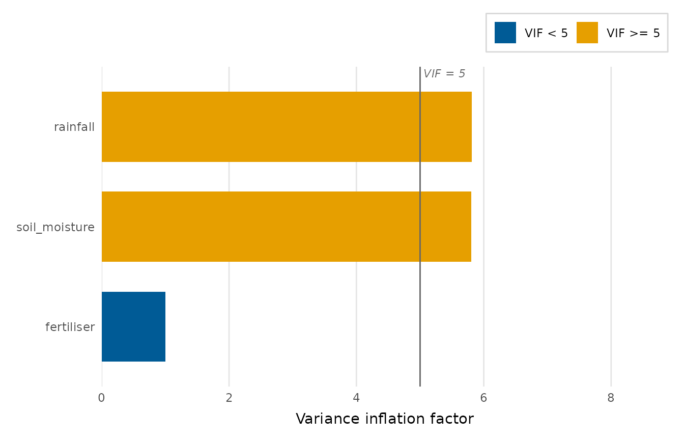
# Two deliberately collinear predictors: soil moisture is largely driven by
# rainfall, so both carry an inflated VIF (around 6, above the line at 5)
# while fertiliser stays near 1.
set.seed(1)
d <- crop_yield
d$soil_moisture <- 0.05 * d$rainfall + rnorm(nrow(d), sd = 2)
vif_plot(lm(yield ~ rainfall + soil_moisture + fertiliser, data = d))
 # Multi-level factors get a single generalised VIF per term
fit2 <- lm(yield ~ rainfall + fertiliser + treatment, data = crop_yield)
vif_plot(fit2)
# Multi-level factors get a single generalised VIF per term
fit2 <- lm(yield ~ rainfall + fertiliser + treatment, data = crop_yield)
vif_plot(fit2)