Show a finished figure as a reader with a colour-vision deficiency sees it

simulate_cvd() simulates a set of colours, and this function the figure they end up in, legend, colourbar, text and background included.

Usage

simulate_figure(plot, deficiency, severity = 1)

Arguments

plot: A ggplot or a patchwork, as it would be saved.
deficiency: The deficiency to simulate: "protan" or "deutan" (the two red-green forms) or "tritan" (blue-yellow).
severity: Severity in [0, 1]. Zero leaves the colours unchanged and one is the full deficiency. Machado et al. publish a matrix for each tenth of severity, which is used as it stands at 0.1, 0.2 and so on. A severity between two tenths takes the linear interpolation of their matrices, as the authors suggest and as the colorspace package does.

Value

A gtable, which grid::grid.draw() draws and save_plot() saves.

Details

The plot is turned into the table of grobs that would be drawn, with ggplot2::ggplotGrob() or, for a patchwork, patchwork::patchworkGrob(). Every colour in that table then goes through simulate_cvd(). That covers the line and fill colours of each grob, at any depth, and each cell of a raster, such as a colourbar, a ggplot2::geom_raster() layer or an image added with ggplot2::annotation_raster(). Each colour keeps its alpha channel. Missing and transparent colours are left as they are, and so are gradient and pattern fills such as grid::linearGradient(), which keep their original colours.

The colours are changed after the plot is built. Changing the colours of the data before it is built would leave the legend keys and any colourbar in their original colours, so the legend would no longer match the figure.

The figure stays vector graphics, so it can be saved at any size. The Python twin's simulate_figure() uses the same matrices but rasterises the figure and simulates its pixels, so it returns an image.

References

Machado GM, Oliveira MM, Fernandes LAF (2009). “A physiologically-based model for simulation of color vision deficiency.” IEEE Transactions on Visualization and Computer Graphics, 15(6), 1291–1298. doi:10.1109/TVCG.2009.113 .

Examples

library(ggplot2)
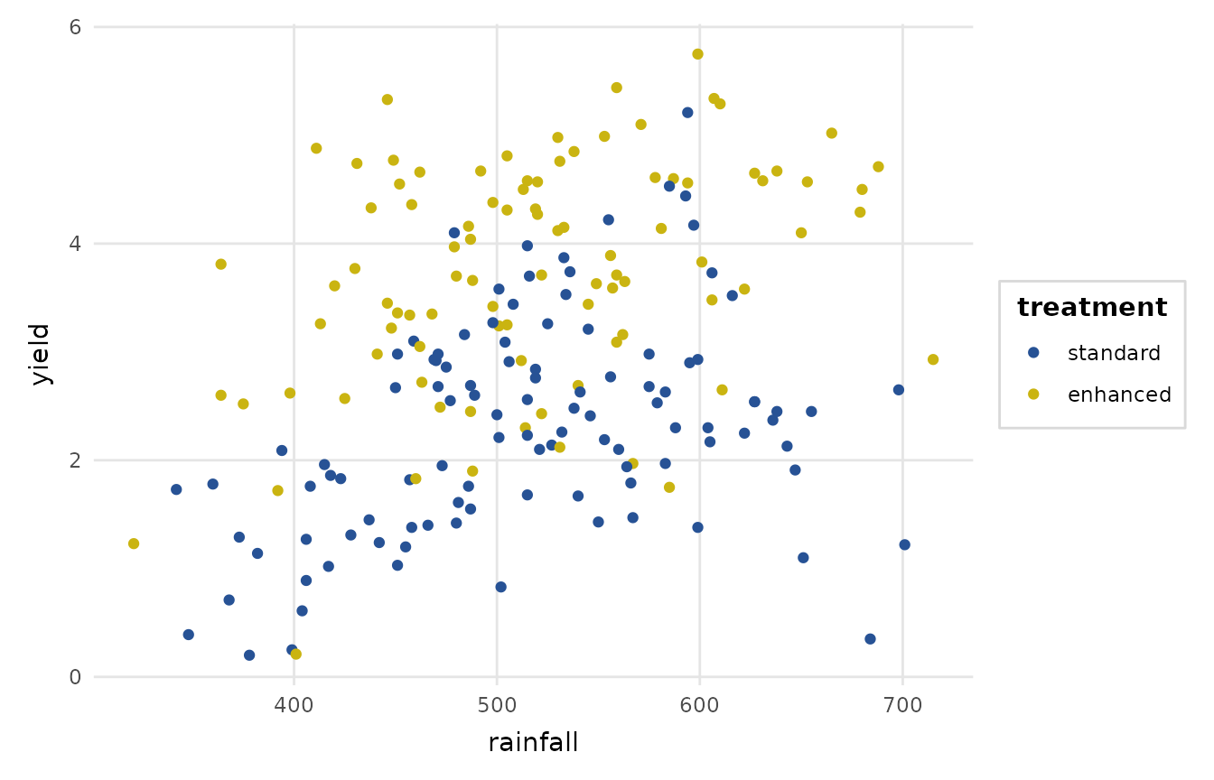
p <- ggplot(crop_yield, aes(rainfall, yield, colour = treatment)) +
  geom_point() +
  scale_colour_depictr() +
  theme_depictr()

# The figure as a reader with deuteranopia sees it.
seen <- simulate_figure(p, "deutan")
grid::grid.newpage()
grid::grid.draw(seen)


# Saved for a side-by-side comparison with the original.
save_plot(file.path(tempdir(), "yield-deutan.png"), seen)