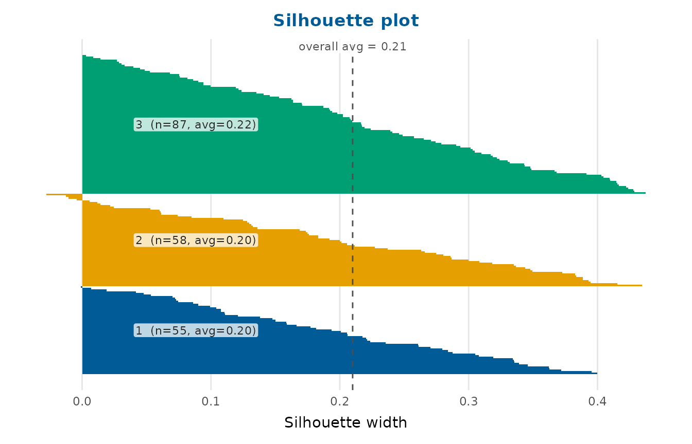
Draws a silhouette plot for a clustering: one horizontal bar per observation, grouped and sorted within cluster, with the average silhouette width shown per cluster and overall. The silhouette width \(s(i)\) compares how close an observation is to its own cluster against the nearest other cluster, and lies in \([-1, 1]\) (higher is better; negative suggests the point may belong to another cluster). It is a standard internal measure of cluster quality.
Usage
silhouette_plot(
  data,
  clusters,
  cols = NULL,
  scale = TRUE,
  distance = "euclidean",
  palette = NULL,
  title = NULL
)
Arguments
- data
A data frame, a numeric matrix, or a stats::dist object.
- clusters
A vector of cluster assignments, one per observation (per row of
data, or matching the objects in adist). Required.- cols
When
datais a data frame, the numeric columns to use (default: all numeric columns).- scale
Whether to scale variables to unit variance before computing the distances (ignored when
datais adist).- distance
Distance measure passed to
stats::dist()(ignored whendatais already adist).- palette
Colours for the clusters; defaults to
depictr_palette().- title
Plot title.
Value
A ggplot2::ggplot object. The per-observation silhouette table is
attached as the attribute "silhouette" and the average width as
"avg_width". The table's cluster and neighbor columns carry the
assignments passed in clusters, as does each band label.
Details
The widths are computed with cluster::silhouette() when the 'cluster'
package is installed, and otherwise with an equivalent base-R implementation,
so the function works with no extra dependency.
References
Rousseeuw PJ (1987). “Silhouettes: A graphical aid to the interpretation and validation of cluster analysis.” Journal of Computational and Applied Mathematics, 20, 53–65. doi:10.1016/0377-0427(87)90125-7 .