Residual-diagnostics panel for a fitted model

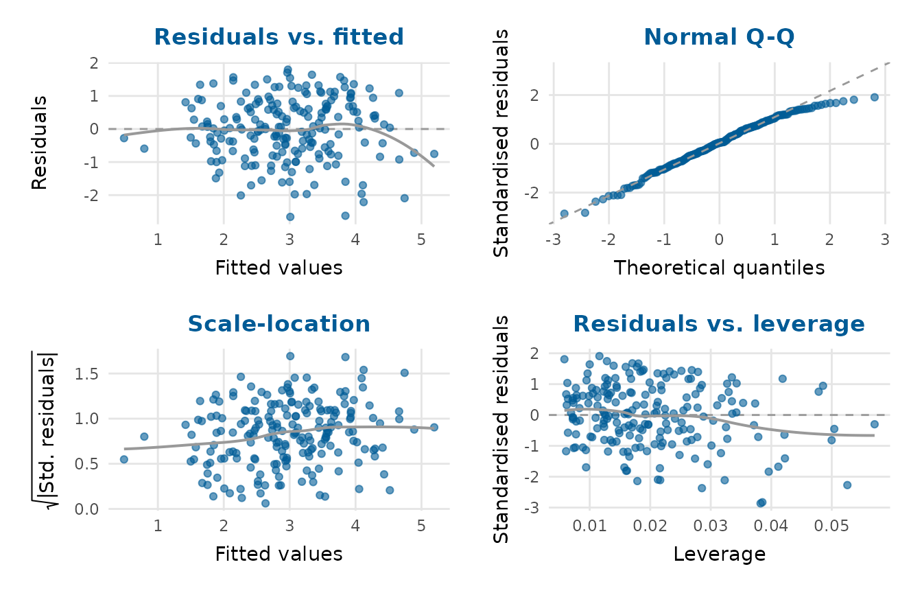
Combines the classic regression diagnostic plots (residuals against fitted values, a normal Q-Q plot of the standardised residuals, a scale-location plot, and residuals against leverage) into a single panel using 'patchwork'. The function works with lm and glm objects.

Usage

residual_diagnostics_plot(
  model,
  which = c("resid_fitted", "qq", "scale_location", "resid_leverage"),
  ncol = 2,
  point_alpha = 0.6,
  smooth = TRUE,
  title = NULL,
  glm_panels = TRUE,
  seed = NULL
)

Arguments

model

A fitted lm or glm model.

which

Character vector choosing which panels to show, any of "resid_fitted", "qq", "scale_location" and "resid_leverage".

ncol

Number of columns in the panel layout.

point_alpha

Point transparency.

smooth

Whether to add a loess guide line to the residual panels.

title

Overall title for the panel.

glm_panels

For a glm, whether to use the GLM-appropriate binned and quantile-residual panels (the default) instead of the classic lm panels. Ignored for an lm.

seed

Optional integer seed for the randomisation of discrete quantile residuals, for reproducible glm Q-Q panels.

Value

A 'patchwork' object (printable like a ggplot2::ggplot).

Details

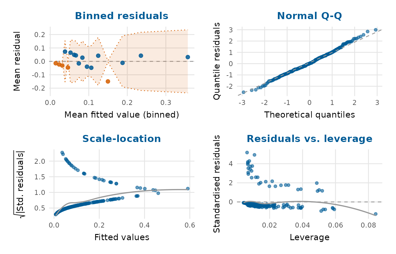
For a glm, the default panels are made GLM-aware (glm_panels = TRUE): the "residuals vs. fitted" panel is replaced by a binned-residual plot (Gelman & Hill, 2007; see binned_residual_plot()), which is readable even for binary or count models, and the Q-Q panel uses randomised quantile residuals (Dunn & Smyth, 1996), which are standard normal under a correctly specified model regardless of the response family. The scale-location and leverage panels are unchanged. For an lm the behaviour is identical to before. Set glm_panels = FALSE to force the classic lm-style panels for a glm as well.

References

Gelman A, Hill J (2007). Data analysis using regression and multilevel/hierarchical models. Cambridge University Press, Cambridge, UK. ISBN 978-0-521-68689-1. doi:10.1017/CBO9780511790942 .

Dunn PK, Smyth GK (1996). “Randomized quantile residuals.” Journal of Computational and Graphical Statistics, 5(3), 236–244. doi:10.1080/10618600.1996.10474708 .

Examples

fit <- lm(yield ~ rainfall + fertiliser + soil_ph, data = crop_yield)
residual_diagnostics_plot(fit)

# \donttest{
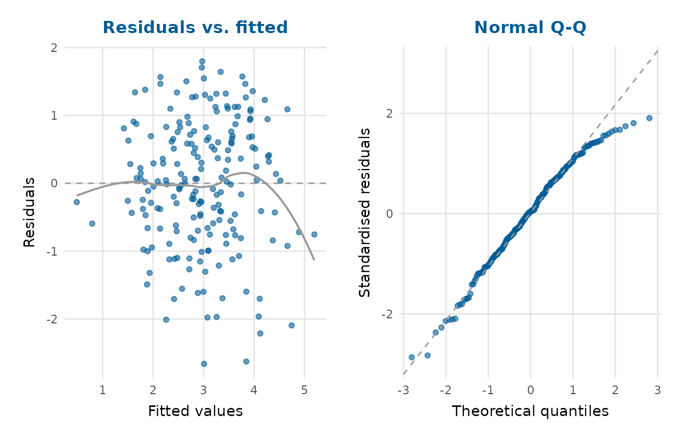
residual_diagnostics_plot(fit, which = c("resid_fitted", "qq"))


# A logistic GLM gets binned and quantile-residual panels automatically:
gfit <- glm(adverse_event ~ biomarker + age + arm,
            data = clinical_trial, family = binomial)
residual_diagnostics_plot(gfit)

# }