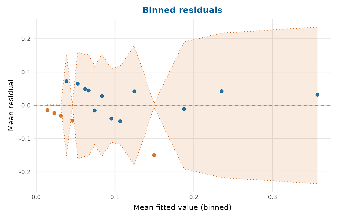
Binned-residual plot for a generalised linear model — binned_residual

For a fitted glm (especially binary or count models), a plot of raw residuals against fitted values is hard to read because the residuals take only a few values. Following Gelman and Hill (2007), this plot instead splits the data into equal-count bins of fitted values and plots, for each bin, the mean residual against the mean fitted value, inside a grey band of $\pm 2$ standard errors of that mean. Under a well-specified model, the binned residuals scatter around zero, and about 95% of them should fall within the band. Systematic departures (a trend, or many points outside the band) indicate a misspecified mean structure.

Usage

binned_residual_plot(
  model,
  bins = NULL,
  type = c("response", "pearson"),
  point_colour = depictr_brand(),
  band_colour = depictr_accent(),
  title = NULL,
  band = c("model", "empirical")
)

Arguments

model: A fitted glm object (an lm is also accepted and treated as a Gaussian GLM).
bins: Number of bins. The default follows Gelman and Hill's rule of thumb of roughly $\sqrt{n}$ bins (bounded to a sensible range).
type: Residual type used for the bin means: "response" (observed minus fitted on the response scale, the Gelman-Hill default) or "pearson".
point_colour, band_colour: Colours for the bin points and the $\pm 2$ SE band. Default to the depictr brand and accent colours.
title: Plot title.
band: Where the standard errors come from. The default, "model", takes them from the variance the fitted model implies for each residual. "empirical" takes them from the spread of the residuals in each bin, as in depictr 0.3.0 and arm::binnedplot().

Value

A ggplot2::ggplot object. The per-bin summary (mean fitted value, mean residual, number of observations n, the band's half-width se2 and an outside flag) is attached as attr(plot, "bins").

Details

By default (band = "model"), the standard error is the one the fitted model implies. The model gives the response $y_i$ the variance $\phi V(\hat\mu_i) / w_i$, where $V$ is the family's variance function, $w_i$ the prior weight and $\phi$ the dispersion. The dispersion is 1 for the binomial and Poisson families, summary(model)$dispersion for the others and $\hat\sigma^2$ for an lm. Taking this as the variance of the response residual $y_i - \hat\mu_i$, the band gives the mean of the $n_b$ residuals in bin $b$ the standard error $\sqrt{\sum_{i \in b} \phi V(\hat\mu_i) / w_i} / n_b$. A Pearson residual, $(y_i - \hat\mu_i) \sqrt{w_i / V(\hat\mu_i)}$, then has variance $\phi$, so its bin mean has standard error $\sqrt{\phi / n_b}$. The fit absorbs a little of each observation's variance, so a residual varies slightly less than this and the band errs on the wide side. Observations with zero prior weight take no part in the fit and are left out of the bins.

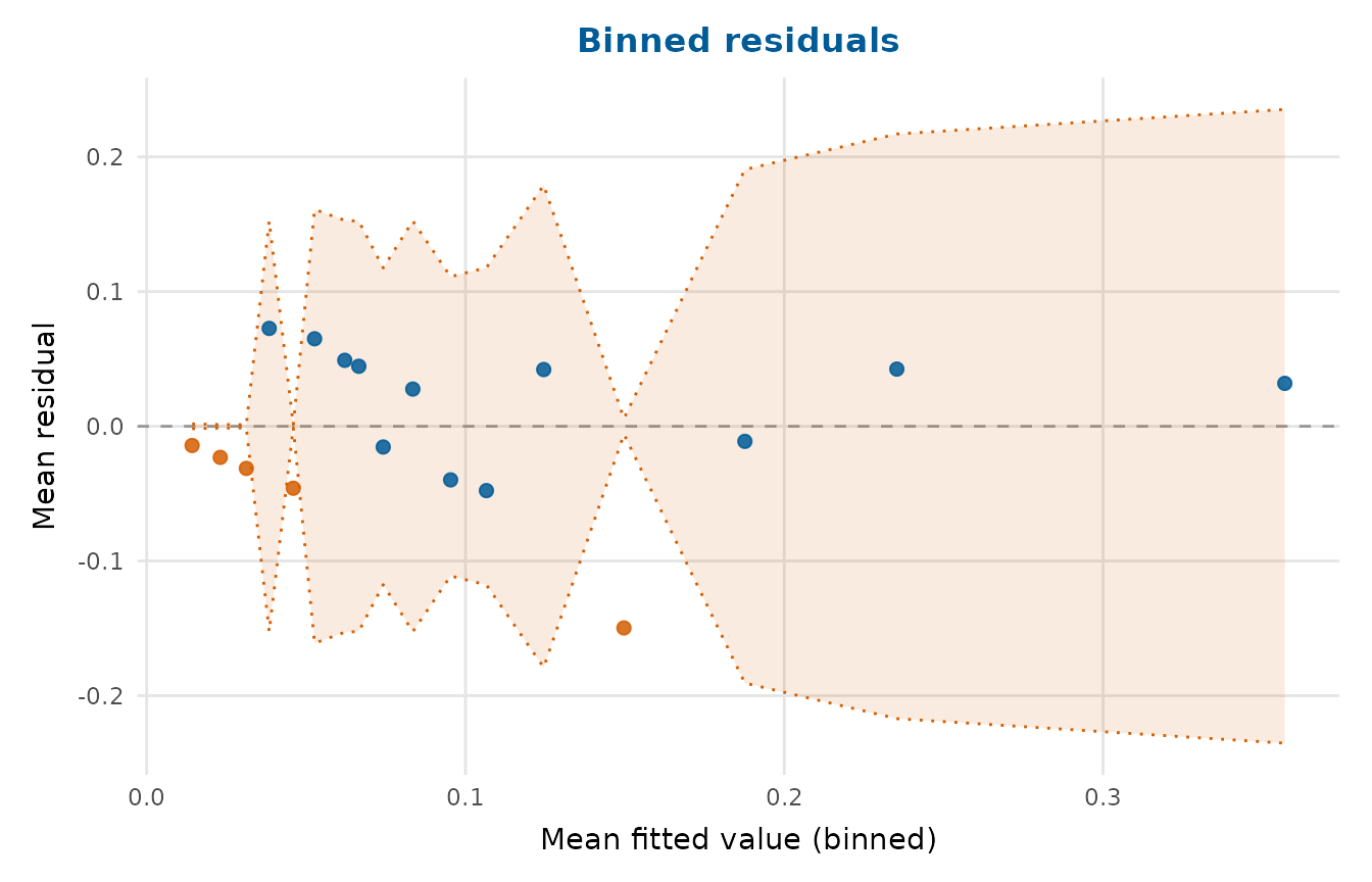
band = "empirical" draws the band of depictr 0.3.0 and earlier, the one arm::binnedplot() draws: twice the standard deviation of the residuals in the bin, divided by $\sqrt{n_b}$. It collapses wherever the outcomes in a bin are all alike. The residuals in a logistic model's bin without events all lie just below zero, so its band nearly vanishes and the bin is flagged. Where events are rare, such bins are what the model expects. The example below, a correctly specified model, has five of its seventeen bins flagged by that band and none by the model's.

References

Gelman A, Hill J (2007). Data analysis using regression and multilevel/hierarchical models. Cambridge University Press, Cambridge, UK. ISBN 978-0-521-68689-1. doi:10.1017/CBO9780511790942 .

Examples

gfit <- glm(adverse_event ~ biomarker + age + arm,
            data = clinical_trial, family = binomial)
binned_residual_plot(gfit)


# The band of depictr 0.3.0, which flags the bins that hold no events:
binned_residual_plot(gfit, band = "empirical")