Normal quantile-quantile plot — qq

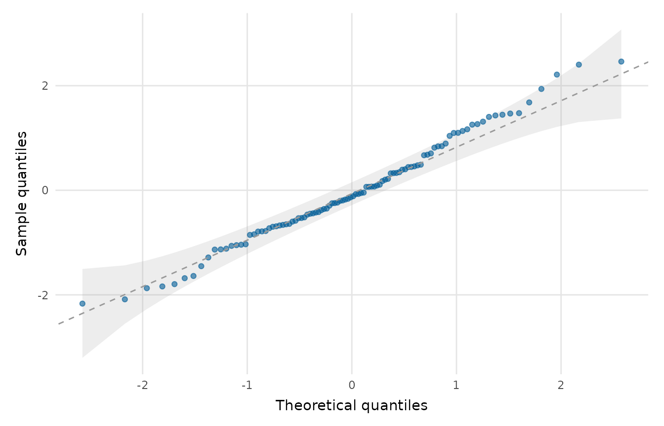
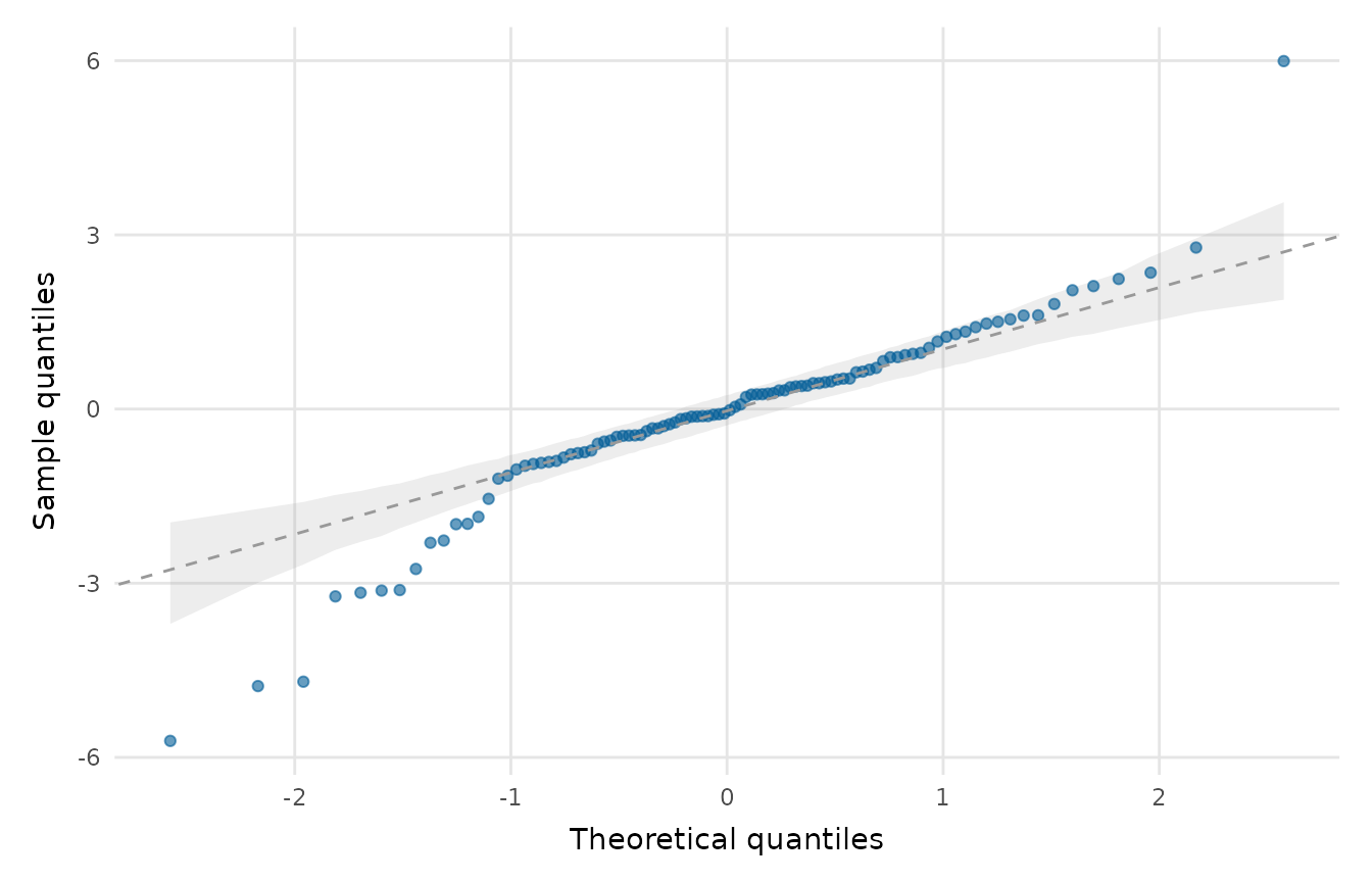
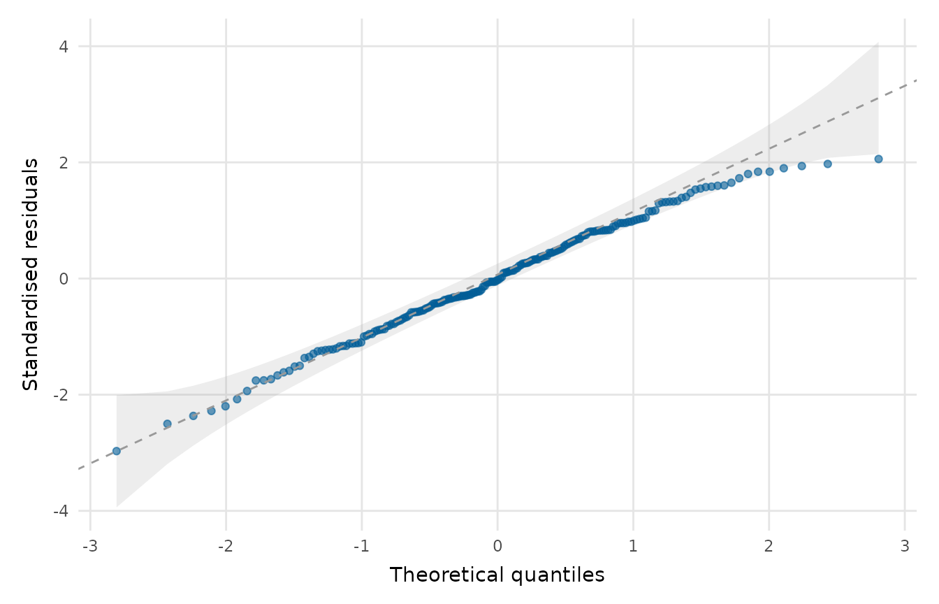
A normal Q-Q plot for a numeric vector or for the standardised residuals of a fitted model, with a reference line and an optional confidence band that makes departures from normality easier to judge. Points that stray outside the band are unusual under normality; under a normal sample roughly level of the points fall inside a pointwise band.

Usage

qq_plot(
  x,
  colour = depictr_brand(),
  title = NULL,
  x_lab = "Theoretical quantiles",
  y_lab = NULL,
  band = TRUE,
  band_type = c("pointwise", "simulate"),
  level = 0.95,
  n_sim = 1000,
  band_fill = depictr_reference(),
  seed = NULL
)

Arguments

x: A numeric vector, or a fitted lm/glm model (its standardised residuals are used).
colour: Point colour. Defaults to the depictr brand blue.
title, x_lab, y_lab: Title and axis labels.
band: Whether to draw a confidence band/envelope.
band_type: Band construction: "pointwise" (analytic order-statistic standard errors, the default) or "simulate" (a Monte-Carlo envelope).
level: Confidence level for the band.
n_sim: Number of simulations for band_type = "simulate".
band_fill: Fill colour of the band.
seed: Optional integer seed for the simulated envelope, for reproducibility.

Value

A ggplot2::ggplot object.

Details

Two band constructions are offered. "pointwise" is analytic: it uses the large-sample standard error of the \(i\)-th order statistic, \(\mathrm{se} = \frac{\hat\sigma}{\phi(z_i)}\sqrt{p_i(1-p_i)/n}\), around the fitted reference line. "simulate" builds a Monte-Carlo envelope by repeatedly drawing normal samples of the same size and taking the empirical quantiles of the simulated order statistics, which needs no large-sample approximation.

Examples

qq_plot(rnorm(100))

qq_plot(rt(100, df = 3), band_type = "simulate")

fit <- lm(yield ~ rainfall + fertiliser, data = crop_yield)
qq_plot(fit)

References

Dunn PK, Smyth GK (1996). “Randomized quantile residuals.” Journal of Computational and Graphical Statistics, 5(3), 236–244. doi:10.1080/10618600.1996.10474708 .