
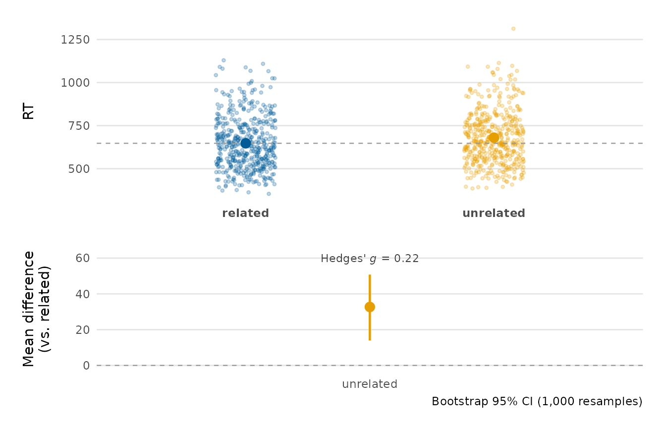
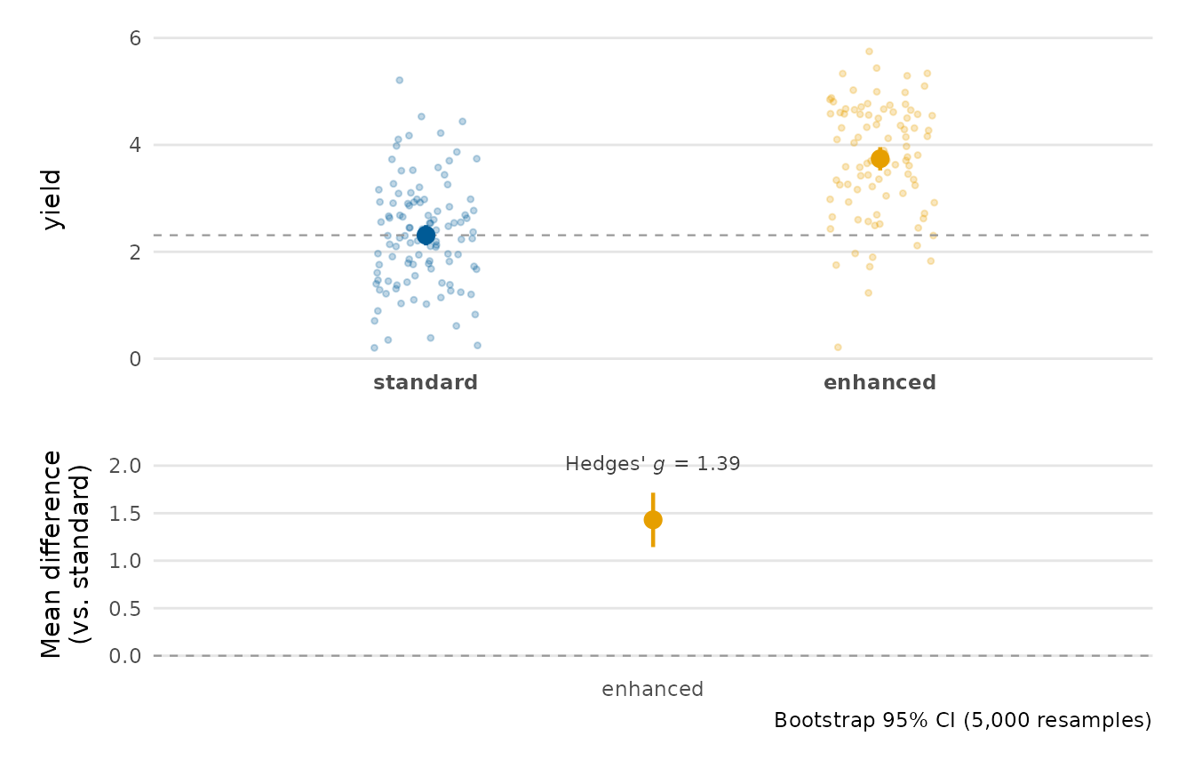
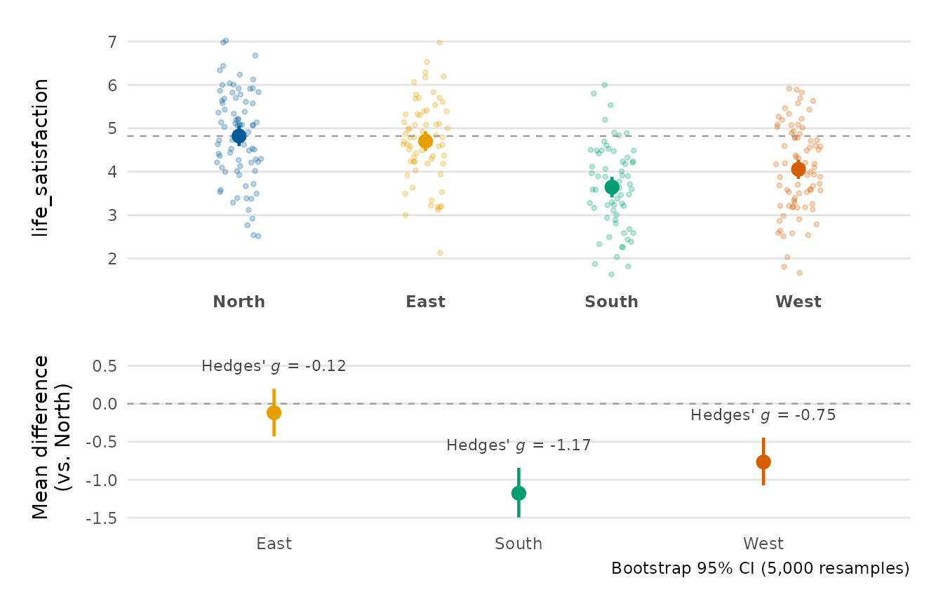
An estimation plot puts the effect size and its uncertainty at the centre of the comparison, rather than a p-value. The upper panel shows each group's raw data (jittered) with its mean and confidence interval. The lower panel shows the difference between each other group's mean and a reference group's mean, with a bootstrap confidence interval. Each difference is drawn in its group's column, beneath that group's data. The two panels are stacked with 'patchwork', and each has its own outcome axis.
Arguments
- data
A data frame.
- y
The numeric outcome (string or unquoted name).
- group
The grouping variable (string or unquoted name).
- reference
The reference (control) group that the others are compared with; defaults to the first level of
group. The reference is drawn first in the upper panel and has an empty column in the lower panel, where the dashed line marks a difference of zero.- conf_level
Confidence level for both the group intervals (t-based) and the bootstrap difference intervals, a single number strictly between 0 and 1.
- n_boot
Number of bootstrap resamples for the difference intervals.
- effsize
Standardised effect size annotated beside each difference:
"hedges_g"(the default, small-sample corrected),"cohens_d", or"none"to omit it. Every contrast against the reference is labelled, so the standardised effect is shown for both the two-group and multi-group cases.- show_points
Whether to draw the raw data behind the group means.
- point_alpha
Transparency of the raw points.
- palette
Colours for the groups; defaults to
depictr_palette().- title, y_lab
Title and outcome-axis label.
- heights
Relative heights of the upper (raw data) and lower (difference) panels, passed to
patchwork::plot_layout().
Value
A 'patchwork' object (printable like a ggplot2::ggplot). The
computed differences and their bootstrap intervals are attached as the
"differences" attribute (a data frame).
Details
This stacked layout is the Cumming estimation plot (Cumming, 2012; Ho et al., 2019), with two groups as with more. Each difference is annotated with a standardised effect size: Cohen's d or, by default, the small-sample corrected Hedges' g (Hedges, 1981). The Gardner-Altman plot (Gardner & Altman, 1986) is a different layout, which sets a single difference beside the two groups on a floating axis whose zero is level with the reference group's mean.
The lower-panel interval is a non-parametric bootstrap of the mean
difference: the two groups are resampled with replacement n_boot times and
the requested percentile interval is read off the resampled differences. This
makes no normality assumption about the sampling distribution of the
difference. The bootstrap uses base R only; set a seed beforehand for
reproducibility.
A group with fewer than two observations has no estimable spread, so its confidence interval is omitted (the mean is still drawn) and a difference involving it is shown as a point without a bootstrap interval; a warning is issued in both cases.
References
Cumming G (2012). Understanding the new statistics: Effect sizes, confidence intervals, and meta-analysis. Routledge, New York, NY. ISBN 978-0-415-87968-2.
Gardner MJ, Altman DG (1986). “Confidence intervals rather than P values: Estimation rather than hypothesis testing.” BMJ, 292(6522), 746–750. doi:10.1136/bmj.292.6522.746 .
Hedges LV (1981). “Distribution theory for Glass's estimator of effect size and related estimators.” Journal of Educational Statistics, 6(2), 107–128. doi:10.3102/10769986006002107 .
Ho J, Tumkaya T, Aryal S, Choi H, Claridge-Chang A (2019). “Moving beyond P values: Data analysis with estimation graphics.” Nature Methods, 16(7), 565–566. doi:10.1038/s41592-019-0470-3 .
Examples
set.seed(1)
# n_boot is kept small here for speed; use the default for real work.
estimation_plot(lexical_decision, RT, condition, n_boot = 1000)
 # \donttest{
estimation_plot(crop_yield, yield, treatment)
# \donttest{
estimation_plot(crop_yield, yield, treatment)
 # More than two groups: differences vs a chosen reference
estimation_plot(wellbeing_survey, life_satisfaction, region,
reference = "North")
# More than two groups: differences vs a chosen reference
estimation_plot(wellbeing_survey, life_satisfaction, region,
reference = "North")
 # }
# }