Time-series decomposition plot

Decomposes a seasonal time series into trend, seasonal and remainder components and shows them, with the original series, as stacked panels.

Usage

decompose_plot(
  x,
  frequency = NULL,
  method = c("stl", "classical"),
  robust = FALSE,
  s_window = "periodic",
  confidence = FALSE,
  level = 0.95,
  title = NULL
)

Arguments

x: A ts object, or a numeric vector (then frequency is required), holding one series. A multivariate ts or a matrix with several columns is refused. Missing values at either end are trimmed, and a missing value inside the series is an error.
frequency: Number of observations per period (e.g. 12 for monthly data); taken from x when it is a ts.
method: "stl" (loess-based, Cleveland et al., 1990) or "classical" (stats::decompose()). STL needs more than two full cycles of data, and classical decomposition at least two.
robust: For method = "stl", whether to fit a robust STL (stats::stl() with robust = TRUE), which down-weights outliers in the loess fits so that an unusual point bleeds less into the trend and seasonal components. Ignored for the classical method.
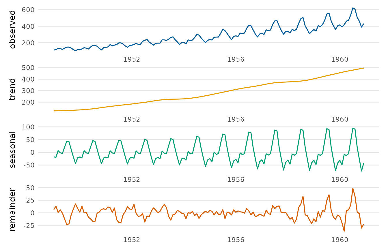
s_window: For method = "stl", the seasonal window, passed to stats::stl() as s.window. The default, "periodic", estimates one seasonal value per position in the cycle and repeats it in every cycle, as classical decomposition does. An odd whole number of at least 7 lets the seasonal component change from cycle to cycle. It is the number of consecutive cycles that go into each seasonal value, so a smaller window lets the pattern change faster. Ignored for the classical method.
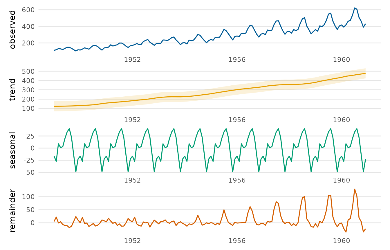
confidence: Whether to draw a confidence ribbon around the trend component. The band is a normal-approximation interval based on the remainder's standard deviation (see Details).
level: Coverage of the trend confidence ribbon (a single number strictly between 0 and 1).
title: Plot title.

Value

A 'patchwork' object (printable like a ggplot2::ggplot).

Details

The trend confidence ribbon is a pragmatic normal-approximation band: trend +/- z * sd(remainder), where z = qnorm((1 + level) / 2) and the remainder standard deviation is computed on the non-missing remainder values. It conveys the scale of the unexplained variation around the smoothed trend rather than a formal sampling-distribution interval.

References

Cleveland RB, Cleveland WS, McRae JE, Terpenning I (1990). “STL: A seasonal-trend decomposition procedure based on loess.” Journal of Official Statistics, 6(1), 3–73.

Examples

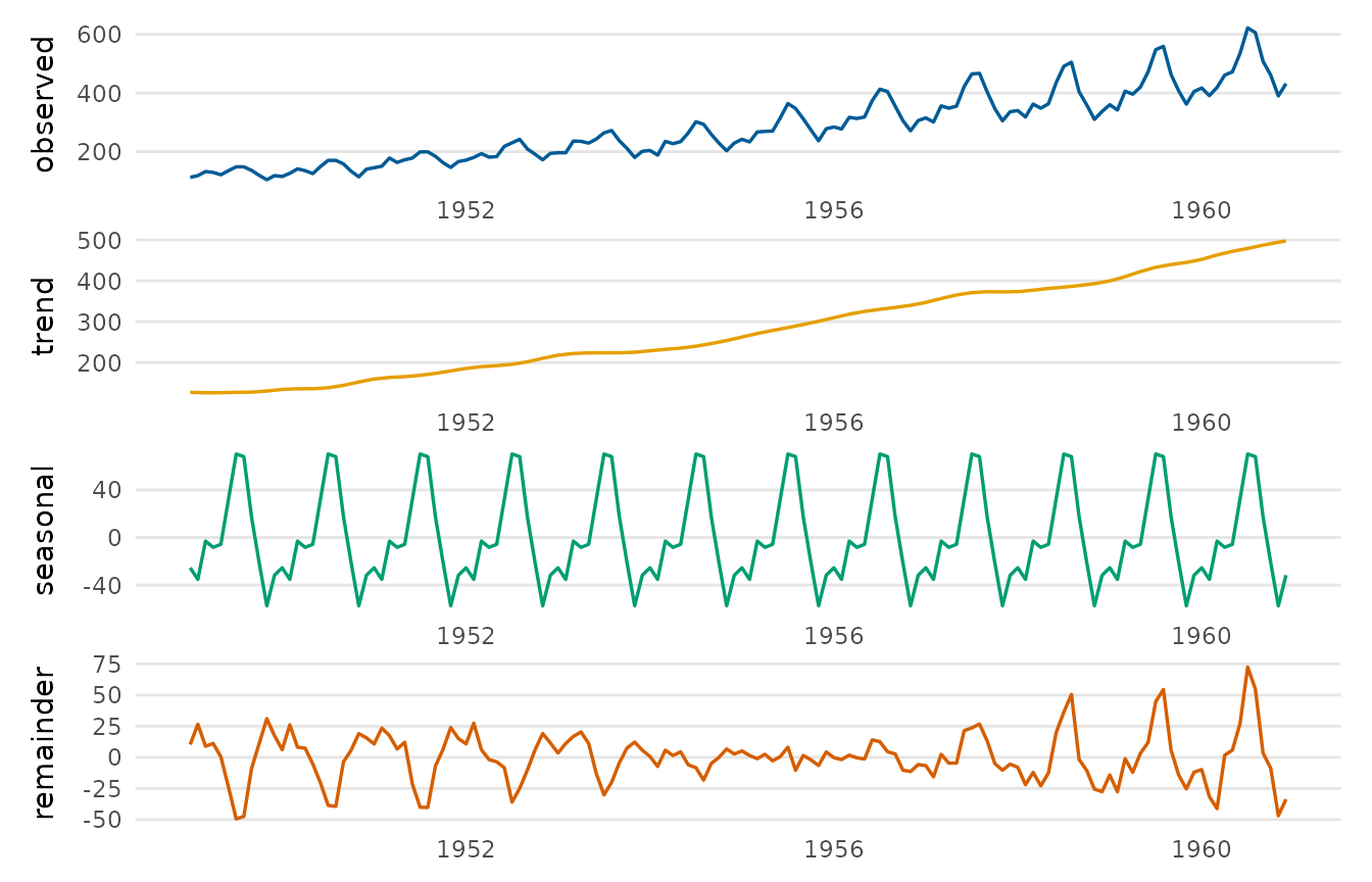
decompose_plot(AirPassengers)

# \donttest{
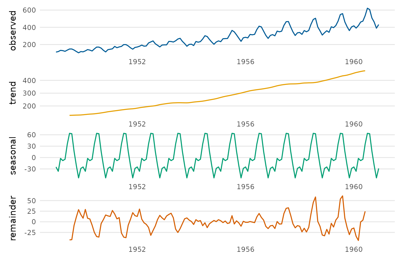
decompose_plot(AirPassengers, method = "classical")

# Robust STL with a confidence ribbon on the trend
decompose_plot(AirPassengers, robust = TRUE, confidence = TRUE)

# A seasonal component free to grow with the level of the series
decompose_plot(AirPassengers, s_window = 13)

# }