Power and design analysis

library(pilotr)

Simulation-based power addresses how often an analysis would detect an effect if the world matched the specification exactly. pilotr estimates this by repeatedly simulating from the ground-truth specification, fitting the analysis model and recording the proportion of significant results. Beyond power, it reports the design-analysis quantities of Gelman and Carlin (2014), namely the Type S (sign) error and the Type M (magnitude, or exaggeration) ratio.

The mixed-effects examples below use small n_sims, and their results were precomputed with exactly the code shown and shipped with the package, so that the vignette builds quickly. For real planning, we recommend n_sims >= 200, with more replicates for stable Type S and Type M estimates.

Two-group Gaussian

The classic case has a closed-form analytic power, which the simulation matches.

spec <- build_spec(list(
  name = "two_group", seed = 1, design_kind = "between", n_subject = 64,
  factor_name = "group", lev1 = "control", lev2 = "treatment",
  intercept = 100, effect = 5, family = "gaussian", resp_name = "score", sigma = 10))

pw <- power_design(spec, n_sims = 500)
unlist(pw[c("power", "type_s", "type_m", "true_effect", "mean_estimate")])
#>         power        type_s        type_m   true_effect mean_estimate 
#>      0.504000      0.000000      1.372571      5.000000      4.947259

At roughly 50% power, the Type M ratio is well above 1. Conditional on significance, the estimated effect is exaggerated, even though the average estimate over all replicates is unbiased. This reflects the statistical-significance filter, which is precisely what design analysis is meant to expose.

Crossed mixed-effects designs

A feature that distinguishes pilotr from a marginal simulator is power estimation for crossed by-subject and by-item designs. The R interface fits the maximal model y ~ cond + (1 + cond | subject) + (1 + cond | item) with lme4/lmerTest and tests the fixed effect with Satterthwaite degrees of freedom.

spec_c <- build_spec(list(
  name = "priming", seed = 1, design_kind = "within", include_items = TRUE,
  n_subject = 24, n_item = 18,
  factor_name = "condition", lev1 = "related", lev2 = "unrelated",
  intercept = 6, effect = 0.06,
  subj_int_sd = 0.12, subj_slope_sd = 0.04, subj_corr = 0.2,
  item_int_sd = 0.08, item_slope_sd = 0.02, item_corr = -0.1,
  family = "shifted_lognormal", resp_name = "RT", sigma = 0.3, shift = 200))

pm <- power_mixed(spec_c, n_sims = 20)   # tiny for the vignette; use >= 200 in practice
unlist(pm[c("power", "type_s", "type_m", "n_converged")])

#>       power      type_s      type_m n_converged 
#>    0.800000    0.000000    1.193659   20.000000

n_converged reports how many replicates the maximal model actually fit. This is a useful diagnostic in its own right, since convergence problems are common in small crossed designs, and it is the denominator of power, which is the significant proportion among the converged replicates.

power_mixed() runs pilotr’s own simulation loop over the portable specification rather than wrapping an existing power package. It covers territory pioneered by simr (Green and MacLeod, 2016) and mixedpower (Kumle, Vo and Draschkow, 2021). pilotr differs in being driven by the cross-language specification, in reporting Type S and Type M errors alongside power, and in built-in parallelisation.

A power curve

The following sweep over the number of subjects shows where power crosses a target.

curve <- power_curve_mixed(spec_c, subject_ns = c(8, 12, 16, 24, 32, 44, 56), n_sims = 50)
curve

#>   n_subject power   type_m n_converged
#> 1         8  0.16 1.998682          50
#> 2        12  0.34 1.639186          50
#> 3        16  0.48 1.404611          50
#> 4        24  0.80 1.189207          50
#> 5        32  0.86 1.129062          50
#> 6        44  0.96 1.046713          50
#> 7        56  0.96 1.048449          50

# The transparent device canvas is what lets the page colour through: a ggplot theme alone
# cannot do it, since the device paints white underneath. The website's dark mode then
# inverts the figure's ink, so the axes and labels follow the theme instead of sitting on
# an opaque matte.
library(ggplot2)
# Each power estimate is a proportion over the converged replicates, so it carries a
# binomial Monte Carlo standard error. The shaded band is the 95% interval.
curve$se <- sqrt(curve$power * (1 - curve$power) / curve$n_converged)
ggplot(curve, aes(n_subject, power)) +
  geom_hline(yintercept = 0.8, linetype = 2, colour = "grey60") +
  geom_ribbon(aes(ymin = pmax(0, power - 1.96 * se), ymax = pmin(1, power + 1.96 * se)),
              alpha = .15, fill = "#2C6FB0") +
  geom_line(colour = "#2C6FB0", linewidth = 0.8) +
  geom_point(colour = "#2C6FB0", size = 2.6) +
  scale_y_continuous(limits = c(0, 1)) +
  labs(x = expression(italic(N) ~ "subjects"), y = "Power") +
  theme_minimal(base_size = 12) +
  # theme_minimal still paints a white plot.background over the transparent canvas, so
  # both surfaces have to be cleared for the page colour to reach the figure. The ink is
  # left at its default: the website inverts the figure in dark mode, which turns the dark
  # axis text light, whereas a fixed mid-grey would be inverted into a muddy tan.
  theme(plot.background  = element_rect(fill = NA, colour = NA),
        panel.background = element_rect(fill = NA, colour = NA),
        panel.grid       = element_line(colour = "grey80"))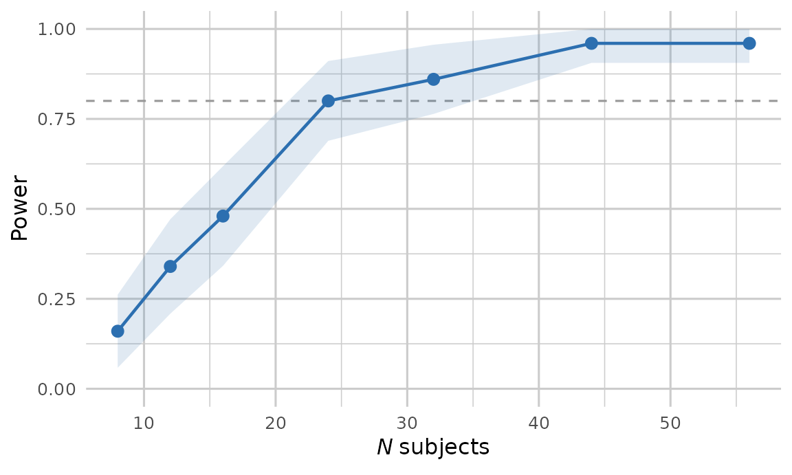

The shaded band shows the Monte Carlo interval, the binomial standard error of each power estimate over its converged replicates widened to a 95% envelope.

Parallel execution

Every power and precision analysis in pilotr takes a workers argument that spreads the Monte Carlo replicates across local cores. Each replicate seeds the shared cross-language RNG from its own index, so the results are identical to a serial run whatever the worker count, and parallelisation costs nothing in reproducibility. The mixed-model fits dominate the running time, which makes the speed-up close to linear in the number of cores. In a sweep the worker pool is created once and reused across all sample sizes.

power_curve_mixed(spec_c, subject_ns = seq(20, 60, 10), n_sims = 500, workers = 8)

This design answers a serial bottleneck familiar from simr::powerCurve(), which this package’s maintainer previously worked around by splitting the sample-size grid across separate jobs by hand and recombining the results afterwards (Bernabeu, 2021). In pilotr the same gain takes one argument.

A bridge to the Bayesian workflow

For a confirmatory Bayesian fit, brms_bridge() emits a ready-to-run brms model. It provides the family, the fixed and random-effects formula, and a weakly-informative prior set, all derived from the same specification, so that the planning model and the confirmatory model remain consistent.

brms_bridge(spec_c)
library(brms)
fit <- brm(
  RT ~ effect + (1 + effect | subject) + (1 + effect | item),
  data   = your_data,
  family = shifted_lognormal(),
  prior  = c(
    prior(normal(0, 2.5), class = "Intercept"),
    prior(normal(0, 0.5), class = "b", coef = "effect"),
    prior(normal(0, 1), class = "sd"),
    prior(lkj(2), class = "cor")
  ),
  chains = 4, iter = 4000, warmup = 2000, cores = 4,
  control = list(adapt_delta = 0.95)
)

Two-group Gaussian

Crossed mixed-effects designs

A power curve

Parallel execution

A bridge to the Bayesian workflow

See also