Plot predicted values for one predictor

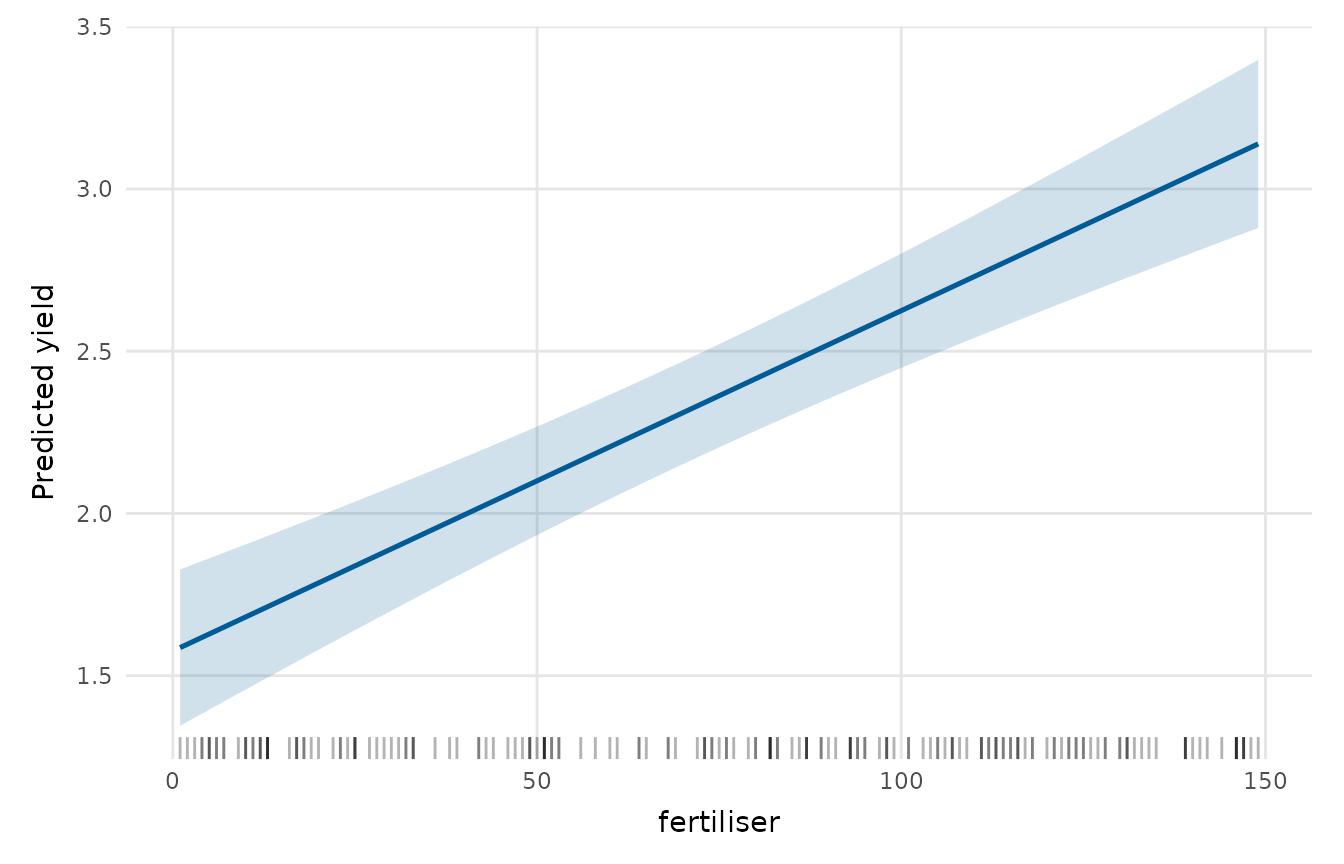
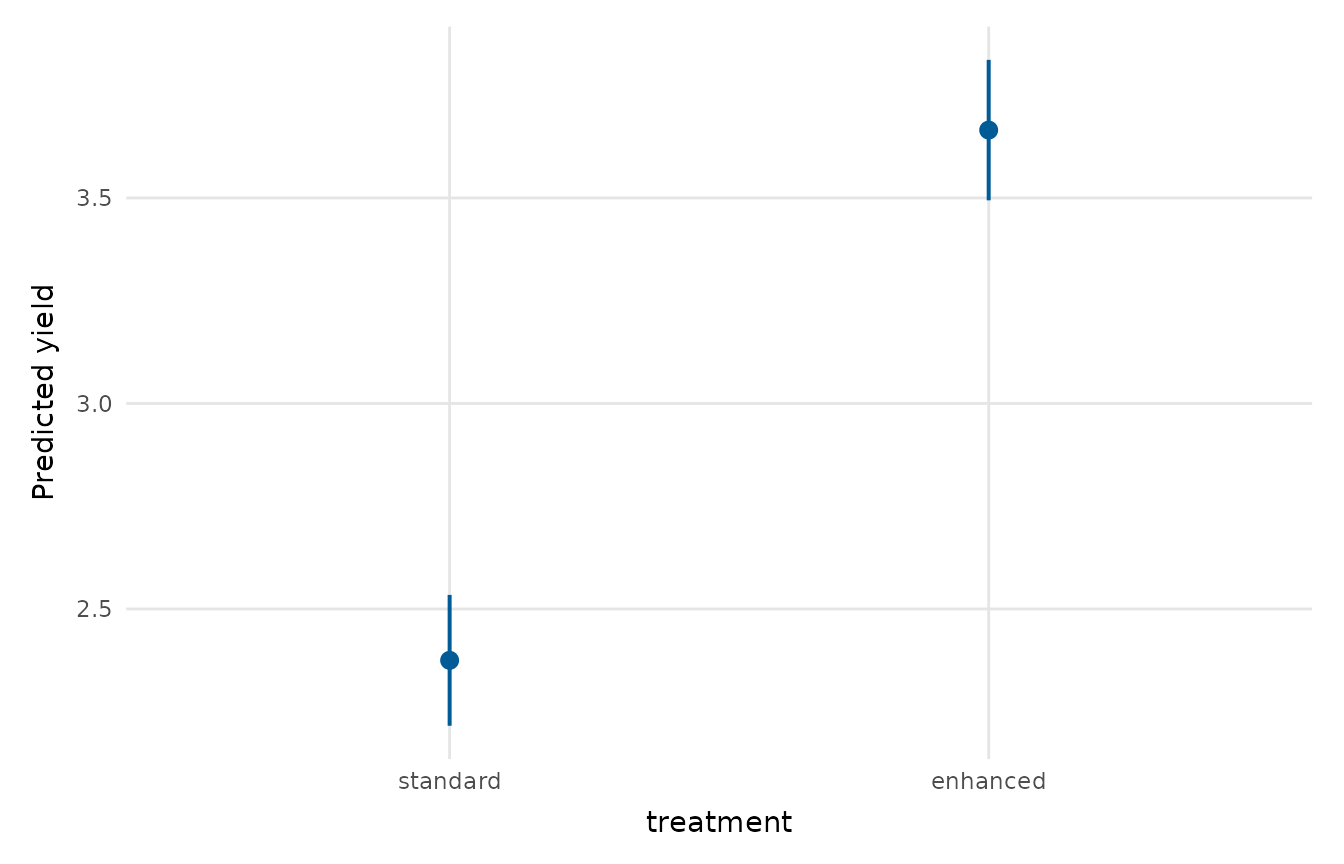
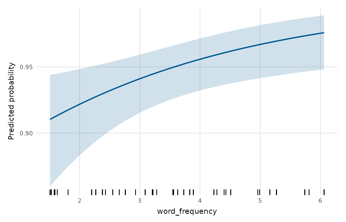
Shows the values a model predicts as one focal predictor varies, holding the other predictors at typical values (the mean for numeric predictors, the most frequent level for factors). A confidence band (numeric predictor) or confidence intervals (factor predictor) convey uncertainty.

Usage

effects_plot(
  model,
  predictor,
  conf_level = 0.95,
  n = 100,
  rug = TRUE,
  colour = depictr_brand(),
  title = NULL,
  x_lab = NULL,
  y_lab = NULL
)

Arguments

model

A fitted model (lm, glm, merMod, ...).

predictor

Name of the focal predictor (string).

conf_level

Confidence level for the interval.

n

Number of points across the range of a numeric predictor.

rug

Whether to add a rug of the observed predictor values (numeric predictors).

colour

Colour for the line/points and band. Defaults to the depictr brand blue.

title, x_lab, y_lab

Title and axis labels.

Value

A ggplot2::ggplot object.

Details

Predictions and standard errors come from stats::predict(); glm predictions are formed on the link scale and back-transformed, so a binomial model shows predicted probabilities. Mixed models fitted with lme4::lmer()/lme4::glmer() are supported too: predictions use only the fixed effects (re.form = NA) and standard errors come from the fixed-effect design matrix and vcov(). Works with lm, glm and merMod; other model classes are attempted on a best-effort basis.

Examples

fit <- lm(yield ~ rainfall + fertiliser + treatment, data = crop_yield)
effects_plot(fit, "fertiliser")

effects_plot(fit, "treatment")


gfit <- glm(accuracy ~ word_frequency + condition,
            data = lexical_decision, family = binomial)
effects_plot(gfit, "word_frequency")        # predicted probability