Why can't we be friends? Plotting frequentist (lmerTest) and Bayesian (brms) mixed-effects models

Visualising frequentist and Bayesian estimates in one plot

Both frequentist and Bayesian statistics offer the options of hypothesis testing and parameter estimation (Cumming, 2014; Kruschke & Liddell, 2018; Rouder et al., 2018; Schmalz et al., 2022; Tendeiro & Kiers, 2019, 2022; van Ravenzwaaij & Wagenmakers, 2022). In the statistical analyses conducted by Bernabeu (2022), hypothesis testing was performed within the frequentist framework, whereas parameter estimation was performed within both the frequentist and the Bayesian frameworks (for other examples of the estimation approach, see Milek et al., 2018; Pregla et al., 2021; Rodríguez-Ferreiro et al., 2020).

Let’s load the function from GitHub and put it to the test.

# Presenting the frequentist and the Bayesian estimates in the same plot. 
# For this purpose, the frequentist results are merged into a plot from 
# brms::mcmc_plot()

source('https://raw.githubusercontent.com/pablobernabeu/language-sensorimotor-simulation-PhD-thesis/main/R_functions/frequentist_bayesian_plot.R')

# install.packages('devtools')
# library(devtools)
# install_version('tidyverse', '1.3.1')  # Due to breaking changes, Version 1.3.1 is required.
# install_version('ggplot2', '3.3.5')  # Due to breaking changes, Version 3.3.5 is required.
library(tidyverse)
library(ggplot2)
library(Cairo)

# Load frequentist coefficients (estimates and confidence intervals)

KR_summary_semanticpriming_lmerTest =
  readRDS(gzcon(url('https://github.com/pablobernabeu/language-sensorimotor-simulation-PhD-thesis/blob/main/semanticpriming/frequentist_analysis/results/KR_summary_semanticpriming_lmerTest.rds?raw=true')))

confint_semanticpriming_lmerTest =
  readRDS(gzcon(url('https://github.com/pablobernabeu/language-sensorimotor-simulation-PhD-thesis/blob/main/semanticpriming/frequentist_analysis/results/confint_semanticpriming_lmerTest.rds?raw=true')))

# Below are the default names of the effects
# rownames(KR_summary_semanticpriming_lmerTest$coefficients)
# rownames(confint_semanticpriming_lmerTest)

# Load Bayesian posterior distributions

semanticpriming_posteriordistributions_weaklyinformativepriors_exgaussian = 
  readRDS(gzcon(url('https://github.com/pablobernabeu/language-sensorimotor-simulation-PhD-thesis/blob/main/semanticpriming/bayesian_analysis/results/semanticpriming_posteriordistributions_weaklyinformativepriors_exgaussian.rds?raw=true')))

# Below are the default names of the effects
# levels(semanticpriming_posteriordistributions_weaklyinformativepriors_exgaussian$data$parameter)


# Reorder the components of interactions in the frequentist results to match 
# with the order present in the Bayesian results.

rownames(KR_summary_semanticpriming_lmerTest$coefficients) =
  rownames(KR_summary_semanticpriming_lmerTest$coefficients) %>%
  str_replace(pattern = 'z_recoded_interstimulus_interval:z_cosine_similarity', 
              replacement = 'z_cosine_similarity:z_recoded_interstimulus_interval') %>%
  str_replace(pattern = 'z_recoded_interstimulus_interval:z_visual_rating_diff', 
              replacement = 'z_visual_rating_diff:z_recoded_interstimulus_interval')

rownames(confint_semanticpriming_lmerTest)  = 
  rownames(confint_semanticpriming_lmerTest) %>%
  str_replace(pattern = 'z_recoded_interstimulus_interval:z_cosine_similarity', 
              replacement = 'z_cosine_similarity:z_recoded_interstimulus_interval') %>%
  str_replace(pattern = 'z_recoded_interstimulus_interval:z_visual_rating_diff', 
              replacement = 'z_visual_rating_diff:z_recoded_interstimulus_interval')


# Create a vector containing the names of the effects. This vector will be passed 
# to the plotting function.

new_labels = 
  
  semanticpriming_posteriordistributions_weaklyinformativepriors_exgaussian$data$parameter %>% 
  unique %>%
  
  # Remove the default 'b_' from the beginning of each effect
  str_remove('^b_') %>%
  
  # Put Intercept in parentheses
  str_replace(pattern = 'Intercept', replacement = '(Intercept)') %>%
  
  # First, adjust names of variables (both in main effects and in interactions)
  str_replace(pattern = 'z_target_word_frequency',
              replacement = 'Target-word frequency') %>%
  str_replace(pattern = 'z_target_number_syllables',
              replacement = 'Number of target-word syllables') %>%
  str_replace(pattern = 'z_word_concreteness_diff',
              replacement = 'Word-concreteness difference') %>%
  str_replace(pattern = 'z_cosine_similarity',
              replacement = 'Language-based similarity') %>%
  str_replace(pattern = 'z_visual_rating_diff',
              replacement = 'Visual-strength difference') %>%
  str_replace(pattern = 'z_attentional_control',
              replacement = 'Attentional control') %>%
  str_replace(pattern = 'z_vocabulary_size',
              replacement = 'Vocabulary size') %>%
  str_replace(pattern = 'z_recoded_participant_gender',
              replacement = 'Gender') %>%
  str_replace(pattern = 'z_recoded_interstimulus_interval',
              replacement = 'SOA') %>%
  # Show acronym in main effect of SOA
  str_replace(pattern = '^SOA$',
              replacement = 'Stimulus onset asynchrony (SOA)') %>%
  
  # Second, adjust order of effects in interactions. In the output from the model, 
  # the word-level variables of interest (i.e., 'z_cosine_similarity' and 
  # 'z_visual_rating_diff') sometimes appeared second in their interactions. For 
  # better consistency, the code below moves those word-level variables (with 
  # their new names) to the first position in their interactions. Note that the 
  # order does not affect the results in any way.
  sub('(\\w+.*):(Language-based similarity|Visual-strength difference)', 
      '\\2:\\1', 
      .) %>%
  
  # Replace colons denoting interactions with times symbols
  str_replace(pattern = ':', replacement = ' × ')


# Create plot
plot_semanticpriming_frequentist_bayesian_plot_weaklyinformativepriors_exgaussian =
  frequentist_bayesian_plot(KR_summary_semanticpriming_lmerTest,
                            confint_semanticpriming_lmerTest,
                            semanticpriming_posteriordistributions_weaklyinformativepriors_exgaussian,
                            labels = new_labels, interaction_symbol_x = TRUE,
                            vertical_line_at_x = 0, x_title = 'Effect size (β)',
                            legend_ncol = 1) + 
  theme(legend.position = 'bottom')

plot_semanticpriming_frequentist_bayesian_plot_weaklyinformativepriors_exgaussian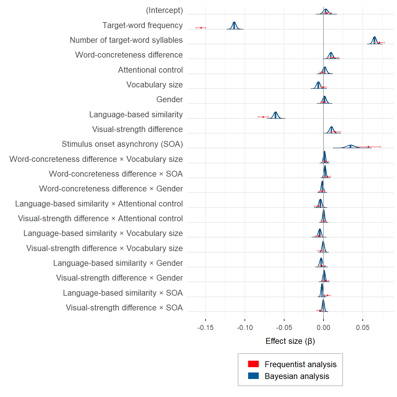

Frequentist and Bayesian estimates are not so polar opposites, are they? What is more, the larger differences between some estimates are the result of the priors that were set on the corresponding effects. With uninformative priors, the frequentist and the Bayesian estimates are virtually identical.

Now it’s time to consider in earnest:

Is frequentist statistics about \(p\) values only? Are frequentist estimates diametrically opposed to Bayesian posterior distributions? Are confidence intervals and credible intervals irreconcilable? Will R crash if lmerTest and brms are simultaneously loaded?

Session info

If you encounter any blockers while reproducing the above analyses using the materials at https://osf.io/gt5uf, my current session info may be useful. For instance, the legend of the plot may not show if the latest versions of the ggplot2 and the tidyverse packages are used. Instead, ggplot2 3.3.5 and tidyverse 1.3.1 should be installed using install_version('ggplot2', '3.3.5') and install_version('tidyverse', '1.3.1').

sessionInfo()

## R version 4.2.3 (2023-03-15 ucrt)
## Platform: x86_64-w64-mingw32/x64 (64-bit)
## Running under: Windows 10 x64 (build 22621)
## 
## Matrix products: default
## 
## locale:
## [1] LC_COLLATE=English_United Kingdom.utf8 
## [2] LC_CTYPE=English_United Kingdom.utf8   
## [3] LC_MONETARY=English_United Kingdom.utf8
## [4] LC_NUMERIC=C                           
## [5] LC_TIME=English_United Kingdom.utf8    
## 
## attached base packages:
## [1] stats     graphics  grDevices utils     datasets  methods   base     
## 
## other attached packages:
##  [1] ggtext_0.1.2        Cairo_1.6-0         forcats_1.0.0      
##  [4] stringr_1.5.0       dplyr_1.1.1         purrr_1.0.1        
##  [7] readr_2.1.4         tidyr_1.3.0         tibble_3.2.1       
## [10] ggplot2_3.3.5       tidyverse_1.3.1     knitr_1.42         
## [13] xaringanExtra_0.7.0
## 
## loaded via a namespace (and not attached):
##  [1] Rcpp_1.0.10      lubridate_1.9.2  digest_0.6.31    utf8_1.2.3      
##  [5] plyr_1.8.8       R6_2.5.1         cellranger_1.1.0 ggridges_0.5.4  
##  [9] backports_1.4.1  reprex_2.0.2     evaluate_0.21    highr_0.10      
## [13] httr_1.4.6       blogdown_1.16    pillar_1.9.0     rlang_1.1.0     
## [17] uuid_1.1-0       readxl_1.4.2     rstudioapi_0.14  jquerylib_0.1.4 
## [21] rmarkdown_2.21   labeling_0.4.2   munsell_0.5.0    gridtext_0.1.5  
## [25] broom_1.0.4      compiler_4.2.3   modelr_0.1.11    xfun_0.38       
## [29] pkgconfig_2.0.3  htmltools_0.5.5  tidyselect_1.2.0 bookdown_0.33.3 
## [33] fansi_1.0.4      crayon_1.5.2     tzdb_0.4.0       dbplyr_2.3.2    
## [37] withr_2.5.0      commonmark_1.9.0 grid_4.2.3       jsonlite_1.8.4  
## [41] gtable_0.3.3     lifecycle_1.0.3  DBI_1.1.3        magrittr_2.0.3  
## [45] scales_1.2.1     cli_3.4.1        stringi_1.7.12   cachem_1.0.7    
## [49] farver_2.1.1     fs_1.6.1         xml2_1.3.3       bslib_0.4.2     
## [53] generics_0.1.3   vctrs_0.6.1      tools_4.2.3      glue_1.6.2      
## [57] markdown_1.5     hms_1.1.3        fastmap_1.1.1    yaml_2.3.7      
## [61] timechange_0.2.0 colorspace_2.1-0 rvest_1.0.3      haven_2.5.2     
## [65] sass_0.4.6

References

Bernabeu, P. (2022). Language and sensorimotor simulation in conceptual processing: Multilevel analysis and statistical power. Lancaster University. https://doi.org/10.17635/lancaster/thesis/1795

Cumming, G. (2014). The new statistics: Why and how. Psychological Science, 25(1), 7–29. https://doi.org/10.1177/0956797613504966

Kruschke, J. K., & Liddell, T. M. (2018). The Bayesian New Statistics: Hypothesis testing, estimation, meta-analysis, and power analysis from a Bayesian perspective. Psychonomic Bulletin & Review, 25(1), 178–206.

Milek, A., Butler, E. A., Tackman, A. M., Kaplan, D. M., Raison, C. L., Sbarra, D. A., Vazire, S., & Mehl, M. R. (2018). “Eavesdropping on happiness” revisited: A pooled, multisample replication of the association between life satisfaction and observed daily conversation quantity and quality. Psychological Science, 29(9), 1451–1462. https://doi.org/10.1177/0956797618774252

Pregla, D., Lissón, P., Vasishth, S., Burchert, F., & Stadie, N. (2021). Variability in sentence comprehension in aphasia in German. Brain and Language, 222, 105008. https://doi.org/10.1016/j.bandl.2021.105008

Rodríguez-Ferreiro, J., Aguilera, M., & Davies, R. (2020). Semantic priming and schizotypal personality: Reassessing the link between thought disorder and enhanced spreading of semantic activation. PeerJ, 8, e9511. https://doi.org/10.7717/peerj.9511

Rouder, J. N., Haaf, J. M., & Vandekerckhove, J. (2018). Bayesian inference for psychology, part IV: Parameter estimation and Bayes factors. Psychonomic Bulletin & Review, 25(1), 102–113. https://doi.org/10.3758/s13423-017-1420-7

Schmalz, X., Biurrun Manresa, J., & Zhang, L. (2021). What is a Bayes factor? Psychological Methods. https://doi.org/10.1037/met0000421

Tendeiro, J. N., & Kiers, H. A. L. (2019). A review of issues about null hypothesis Bayesian testing. Psychological Methods, 24(6), 774–795. https://doi.org/10.1037/met0000221

Tendeiro, J. N., & Kiers, H. A. L. (2022). On the white, the black, and the many shades of gray in between: Our reply to van Ravenzwaaij and Wagenmakers (2021). Psychological Methods, 27(3), 466–475. https://doi.org/10.1037/met0000505

van Ravenzwaaij, D., & Wagenmakers, E.-J. (2022). Advantages masquerading as “issues” in Bayesian hypothesis testing: A commentary on Tendeiro and Kiers (2019). Psychological Methods, 27(3), 451–465. https://doi.org/10.1037/met0000415