Dutch modality exclusivity norms
How it works
exclusivity norms data"] --> B["Flexdashboard front-end
(R Markdown)"] B --> C["Shiny back-end
(reactive selection and download)"] C --> D["Info tab: HTML and CSS text
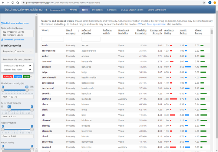
plus rmarkdown output"] C --> E["Table tab: reactable
(colours, bar charts)"] C --> F["Plot tab: plotly
(PCA scatter, tooltips)"] B --> G["Static Flexdashboard-only version
on RPubs (Shiny removed)"]
A nice find was the 'reactable' package, which implements Javascript under the hood to allow the use of colours, bar charts, etc.
Auditory = colDef(header = with_tooltip('Auditory Rating',
                                        'Mean rating of each word on the auditory modality across participants.'),
                  cell = function(value) {
                    width <- paste0(value / max(table_data$Auditory) * 100, "%")
                    value = sprintf("%.2f", round(value,2))  # Round to two digits, keeping trailing zeros
                    bar_chart(value, width = width, fill = '#ff3030')
                    },
                  align = 'left'),
One of the hardest nuts to crack was allowing the full functionality of tables—i.e., scaling to screen, frozen header, and vertical and horizontal scrolling—whilst having tweaked the vertical/horizontal orientation of the dashboard sections. Initial clashes were resolved by adjusting the section's CSS styles
Table {#table style="background-color:#FCFCFC;"}
=======================================================================

Inputs {.sidebar style='position:fixed; padding-top: 65px; padding-bottom:30px;'}
-----------------------------------------------------------------------
and by also adjusting the reactable settings.
renderReactable({
  reactable(selected_words(),
            defaultSorted = list(cat = 'desc', word = 'asc'),
            defaultColDef = colDef(footerStyle = list(fontWeight = "bold")),
            height = 840, striped = TRUE, pagination = FALSE, highlight = TRUE,
A nice feature, especially suited to Flexdashboard, was the use of different formats across tabs. Whereas the Info tab presents long text using HTML and CSS styling, along with rmarkdown code output, the other tabs rely more strongly on Javascript features, enabled by R packages such as ‘shiny’ and sweetalert (e.g., allowing modal dialogs—pop-ups), reactable and plotly (e.g., allowing information opened by hovering—tooltips).
```{r}

# reactive for the word bar
highlighted_properties = reactive(input$highlighted_properties)

renderPlotly({
 ggplotly(
  ggplot( selected_props(), aes(RC1, RC2, label = as.character(word), color = main,
    # Html tags below used for format. Decimals rounded to two.
    text = paste0(' ', '<span style="padding-top:3px; padding-bottom:3px; font-size:2.2em; color:#EEEEEE">', capitalize(word), '</span> ', '<br>',
     '</b><br><span style="color:#EEEEEE"> Dominant modality: </span><b style="color:#EEEEEE">', main, ' ',
     ' ', '</b><br><span style="color:#EEEEEE"> Modality exclusivity: </span><b style="color:#EEEEEE">', sprintf("%.2f", round(Exclusivity, 2)), '% ',
     '</b><br><span style="color:#EEEEEE"> Perceptual strength: </span><b style="color:#EEEEEE">', sprintf("%.2f", round(Perceptualstrength, 2)),
     '</b><br><span style="color:#EEEEEE"> Auditory rating: </span><b style="color:#EEEEEE">', sprintf("%.2f", round(Auditory, 2)), ' ',
     '</b><br><span style="color:#EEEEEE"> Haptic rating: </span><b style="color:#EEEEEE">', sprintf("%.2f", round(Haptic, 2)), ' ',
     '</b><br><span style="color:#EEEEEE"> Visual rating: </span><b style="color:#EEEEEE">', sprintf("%.2f", round(Visual, 2)), ' ',
     '</b><br><span style="color:#EEEEEE"> Concreteness (Brysbaert et al., 2014): </span><b style="color:#EEEEEE">',
       sprintf("%.2f", round(concrete_Brysbaertetal2014, 2)), ' ',
     '</b><br><span style="color:#EEEEEE"> Number of letters: </span><b style="color:#EEEEEE">', letters, ' ',
     '</b><br><span style="color:#EEEEEE"> Number of phonemes (DutchPOND): </span><b style="color:#EEEEEE">',
     round(phonemes_DUTCHPOND, 2), ' ',
     '</b><br><span style="color:#EEEEEE"> Contextual diversity (lg10CD SUBTLEX-NL): </span><b style="color:#EEEEEE">',
       sprintf("%.2f", round(freq_lg10CD_SUBTLEXNL, 2)), ' ',
     '</b><br><span style="color:#EEEEEE"> Word frequency (lg10WF SUBTLEX-NL): </span><b style="color:#EEEEEE">',
       sprintf("%.2f", round(freq_lg10WF_SUBTLEXNL, 2)), ' ',
     '</b><br><span style="color:#EEEEEE"> Lemma frequency (CELEX): </span><b style="color:#EEEEEE">',
       sprintf("%.2f", round(freq_CELEX_lem, 2)), ' ',
     '</b><br><span style="color:#EEEEEE"> Phonological neighbourhood size (DutchPOND): </span><b style="color:#EEEEEE">',
     round(phon_neighbours_DUTCHPOND, 2), ' ',
     '</b><br><span style="color:#EEEEEE"> Orthographic neighbourhood size (DutchPOND): </span><b style="color:#EEEEEE">',
     round(orth_neighbours_DUTCHPOND, 2), ' ',
     '</b><br><span style="color:#EEEEEE"> Age of acquisition (Brysbaert et al., 2014): </span><b style="color:#EEEEEE">',
     sprintf("%.2f", round(AoA_Brysbaertetal2014, 2)), ' ', '<br> '
     ) ) ) +
  geom_text(size = ifelse(selected_props()$word %in% highlighted_properties(), 7,
             ifelse(is.null(highlighted_properties()), 3, 2.8)),
      fontface = ifelse(selected_props()$word %in% highlighted_properties(), 'bold', 'plain')) +
geom_point(alpha = 0) +  # This geom_point helps to colour the tooltip according to the dominant modality
scale_colour_manual(values = colours, drop = FALSE) + theme_bw() + ggtitle('Property words') +
labs(x = 'Varimax-rotated Principal Component 1', y = 'Varimax-rotated Principal Component 2') +
guides(color = guide_legend(title = 'Main<br>modality')) +
theme( plot.background = element_blank(), panel.grid.major = element_blank(),
   panel.grid.minor = element_blank(), panel.border = element_blank(),
   axis.line = element_line(color = 'black'), plot.title = element_text(size = 14, hjust = .5),
   axis.title.x = element_text(colour = 'black', size = 12, margin = margin(15,15,0,15)),
   axis.title.y = element_text(colour = 'black', size = 12, margin = margin(0,15,15,5)),
   axis.text.x = element_text(size = 8), axis.text.y  = element_text(size = 8),
   legend.background = element_rect(size = 2), legend.position = 'none',
 legend.title = element_blank(),
 legend.text = element_text(colour = colours, size = 13) ),
tooltip = 'text'
)
})

# For download, save plot without the interactive 'plotly' part

properties_png = reactive({ ggplot(selected_props(), aes(RC1, RC2, color = main, label = as.character(word))) +
geom_text(show.legend = FALSE, size = ifelse(selected_props()$word %in% highlighted_properties(), 7,
         ifelse(is.null(highlighted_properties()), 3, 2.8)),
      fontface = ifelse(selected_props()$word %in% highlighted_properties(), 'bold', 'plain')) +
geom_point(alpha = 0) + scale_colour_manual(values = colours, drop = FALSE) + theme_bw() +
guides(color = guide_legend(title = 'Main<br>modality', override.aes = list(size = 7, alpha = 1))) +
ggtitle( paste0('Properties', ' (showing ', nrow(selected_props()), ' out of ', nrow(props), ')') ) +
labs(x = 'Varimax-rotated Principal Component 1', y = 'Varimax-rotated Principal Component 2') +
theme( plot.background = element_blank(), panel.grid.major = element_blank(),
   panel.grid.minor = element_blank(), panel.border = element_blank(),
   axis.line = element_line(color = 'black'), plot.title = element_text(size = 17, hjust = .5, margin = margin(3,3,7,3)),
   axis.title.x = element_text(colour = 'black', size = 12, margin = margin(10,10,2,10)),
   axis.title.y = element_text(colour = 'black', size = 12, margin = margin(10,10,10,5)),
   axis.text.x = element_text(size = 8), axis.text.y  = element_text(size = 8),
   legend.background = element_rect(size = 2), legend.position = 'right',
   legend.title = element_blank(), legend.text = element_text(size = 15))
})

```
The only instance in which I drew on JavaScript code outside R packages was to enable tooltips beyond the packages’ limits—for instance, in the sidebar. This JavaScript feature is created at the top of the script, in the head area.
<!-- Javascript function to enable a hovering tooltip -->
<script>
$(document).ready(function(){
   $('[data-toggle="tooltip1"]').tooltip();
});
</script>
In the sidebar, I added a reactive mean for each variable, complementing the range selector.
reactive(cat(paste0('Mean = ',
  sprintf("%.2f", round(mean(selected_words()$Exclusivity),2)))))
Static version published on RPubs
A reduced,
static version was also created to increase the availability of the content. Removing some reactivity features allows the dashboard to be published as a standard website (i.e., on a personal website, on
RPubs, etc.), without the need for a back-end Shiny server. Note that this type of website is dubbed 'static', but it can retain multiple interactive features thanks to Javascript-based tools under the hood, allowed by R packages such as leaflet for maps, DT for tables, plotly for plots, etc.
To create the Flexdashboard-only version departing from the Flexdashboard-Shiny version, I deleted runtime: shiny from the YAML header, and disabled Shiny reactive inputs and objects, as below.
```{r}
# Number of words selected on sidebar
# reactive(cat(paste0('Words selected below: ', nrow(selected_props()))))
```
Reference
Bernabeu, P. (2018). Dutch modality exclusivity norms for 336 properties and 411 concepts [Web application]. Retrieved from https://pablobernabeu.shinyapps.io/Dutch-Modality-Exclusivity-Norms