Bayesian workflow: Prior determination, predictive checks and sensitivity analyses
library(dplyr)
library(ggplot2)
library(ggridges)
library(ggtext)
library(patchwork)
library(papaja)
This post presents a code-through of a Bayesian workflow in R, which can be reproduced using the materials at https://osf.io/gt5uf. The content is closely based on Bernabeu (2022), which was in turn based on lots of other references. In addition to those, you may wish to consider Nicenboim et al. (n.d.), a book in preparation that is already available online (https://vasishth.github.io/bayescogsci/book).
In Bernabeu (2022), a Bayesian analysis was performed to complement the estimates that had been obtained in the frequentist analysis. Whereas the goal of the frequentist analysis had been hypothesis testing, for which \(p\) values were used, the goal of the Bayesian analysis was parameter estimation. Accordingly, we estimated the posterior distribution of every effect, without calculating Bayes factors (for other examples of the same estimation approach, see Milek et al., 2018; Pregla et al., 2021; Rodríguez-Ferreiro et al., 2020; for comparisons between estimation and hypothesis testing, see Cumming, 2014; Kruschke & Liddell, 2018; Rouder et al., 2018; Schmalz et al., 2021; Tendeiro & Kiers, 2019, in press; van Ravenzwaaij & Wagenmakers, 2021). In the estimation approach, the estimates are interpreted by considering the position of their credible intervals in relation to the expected effect size. That is, the closer an interval is to an effect size of 0, the smaller the effect of that predictor. For instance, an interval that is symmetrically centred on 0 indicates a very small effect, whereas—in comparison—an interval that does not include 0 at all indicates a far larger effect.
This analysis served two purposes: first, to ascertain the interpretation of the smaller effects—which were identified as unreliable in the power analyses—, and second, to complement the estimates obtained in the frequentist analysis. The latter purpose was pertinent because the frequentist models presented convergence warnings—even though it must be noted that a previous study found that frequentist and Bayesian estimates were similar despite convergence warnings appearing in the frequentist analysis (Rodríguez-Ferreiro et al., 2020). Furthermore, the complementary analysis was pertinent because the frequentist models presented residual errors that deviated from normality—even though mixed-effects models are fairly robust to such a deviation (Knief & Forstmeier, 2021; Schielzeth et al., 2020). Owing to these precedents, we expected to find broadly similar estimates in the frequentist analyses and in the Bayesian ones. Across studies, each frequentist model has a Bayesian counterpart, with the exception of the secondary analysis performed in Study 2.1 (semantic priming) that included vision-based similarity as a predictor. The R package ‘brms’, Version 2.17.0, was used for the Bayesian analysis (Bürkner, 2018; Bürkner et al., 2022).
Priors
Priors are one of the hardest nuts to crack in Bayesian statistics. First, it can be useful to inspect what priors can be set in the model. Second, it is important to visualise a reasonable set of priors based on the available literature or any other available sources. Third, just before fitting the model, the adequacy of a range of priors should be assessed using prior predictive checks. Fourth, posterior predictive checks were performed to assess the consistency between the observed data and new data predicted by the posterior distributions. Fifth, the influence of the priors on the results should be assessed through a prior sensitivity analysis (Lee & Wagenmakers, 2014; Van de Schoot et al., 2021; also see Bernabeu, 2022; Pregla et al., 2021; Rodríguez-Ferreiro et al., 2020; Stone et al., 2020; Stone et al., 2021).
1. Checking what priors can be set
The brms::get_prior function can be used to check what effects in the model can be assigned a prior. The output (see example) will include the current (perhaps default) prior on each effect.
2. Determining the priors
The priors were established by inspecting the effect sizes obtained in previous studies as well as the effect sizes obtained in our frequentist analyses of the present data (reported in Studies 2.1, 2.2 and 2.3). In the first regard, the previous studies that were considered were selected because the experimental paradigms, variables and analytical procedures they had used were similar to those used in our current studies. Specifically, regarding paradigms, we sought studies that implemented: (I) semantic priming with a lexical decision task—as in Study 2.1—, (II) semantic decision—as in Study 2.2—, or (III) lexical decision—as in Study 2.3. Regarding analytical procedures, we sought studies in which both the dependent and the independent variables were \(z\)-scored. We found two studies that broadly matched these criteria: Lim et al. (2020) (see Table 5 therein) and Pexman & Yap (2018) (see Tables 6 and 7 therein). Out of these studies, Pexman & Yap (2018) contained the variables that were most similar to ours, which included vocabulary size (labelled ‘NAART’) and word frequency.
Based on both these studies and on the frequentist analyses, a range of effect sizes was identified that spanned between β = -0.30 and β = 0.30. This range was centred around 0 as the variables were \(z\)-scored. The bounds of this range were determined by the largest effects, which appeared in Pexman & Yap (2018). Pexman et al. conducted a semantic decision study, and split the data set into abstract and concrete words. The two largest effects they found were—first—a word concreteness effect in the concrete-words analysis of β = -0.41, and—second—a word concreteness effect in the abstract-words analysis of β = 0.20. Unlike Pexman et al., we did not split the data set into abstract and concrete words, but analysed these sets together. Therefore, we averaged between the aforementioned values, obtaining a range between β = -0.30 and β = 0.30.
In the results of Lim et al. (2020) and Pexman & Yap (2018), and in our frequentist results, some effects consistently presented a negative polarity (i.e., leading to shorter response times), whereas some other effects were consistently positive. We incorporated the direction of effects into the priors only in cases of large effects that had presented a consistent direction (either positive or negative) in previous studies and in our frequentist analyses in the present studies. These criteria were matched by the following variables: word frequency—with a negative direction, as higher word frequency leads to shorter RTs (Brysbaert et al., 2016; Brysbaert et al., 2018; Lim et al., 2020; Mendes & Undorf, 2021; Pexman & Yap, 2018)—, number of letters and number of syllables—both with positive directions (Barton et al., 2014; Beyersmann et al., 2020; Pexman & Yap, 2018)—, and orthographic Levenshtein distance—with a positive direction (Cerni et al., 2016; Dijkstra et al., 2019; Kim et al., 2018; Yarkoni et al., 2008). We did not incorporate information about the direction of the word concreteness effect, as this effect can follow different directions in abstract and concrete words (Brysbaert et al., 2014; Pexman & Yap, 2018), and we analysed both sets of words together. In conclusion, the four predictors that had directional priors were covariates. All the other predictors had priors centred on 0. Last, as a methodological matter, it is noteworthy that most of the psycholinguistic studies applying Bayesian analysis have not incorporated any directional information in priors (e.g., Pregla et al., 2021; Rodríguez-Ferreiro et al., 2020; Stone et al., 2020; cf. Stone et al., 2021).
Prior distributions
The choice of priors can influence the results in consequential ways. To assess the extent of this influence, prior sensitivity analyses have been recommended. These analyses are performed by comparing the effect of more and less strict priors—or, in other words, priors varying in their degree of informativeness. The degree of variation is adjusted through the standard deviation, and the means are not varied (Lee & Wagenmakers, 2014; Stone et al., 2020; Van de Schoot et al., 2021).
In this way, we compared the results obtained using ‘informative’ priors (\(SD\) = 0.1), ‘weakly-informative’ priors (\(SD\) = 0.2) and ‘diffuse’ priors (\(SD\) = 0.3). These standard deviations were chosen so that around 95% of values in the informative priors would fall within our initial range of effect sizes that spanned from -0.30 to 0.30. All priors are illustrated in the figure below. These priors resembled others from previous psycholinguistic studies (Pregla et al., 2021; Stone et al., 2020; Stone et al., 2021). For instance, Stone et al. (2020) used the following priors: \(Normal\)(0, 0.1), \(Normal\)(0, 0.3) and \(Normal\)(0, 1). The range of standard deviations we used—i.e., 0.1, 0.2 and 0.3—was narrower than those of previous studies because our dependent variable and our predictors were \(z\)-scored, resulting in small estimates and small \(SD\)s (see Lim et al., 2020; Pexman & Yap, 2018). These priors were used on the fixed effects and on the standard deviation parameters of the fixed effects. For the correlations among the random effects, an \(LKJ\)(2) prior was used (Lewandowski et al., 2009). This is a ‘regularising’ prior, as it assumes that high correlations among random effects are rare (also used in Rodríguez-Ferreiro et al., 2020; Stone et al., 2020; Stone et al., 2021; Vasishth et al., 2018).
# Set seed number to ensure exact reproducibility
# of the random distributions
set.seed(123)
# The code below plots all our types of priors. Each distribution
# contains 10,000 simulations, resulting in 90,000 rows.
# The green vertical rectangle shows the range of plausible effect
# sizes based on previous studies that applied a similar analysis
# (Lim et al., 2020, https://doi.org/10.1177/1747021820906566;
# Pexman & Yap, 2018, https://doi.org/10.1037/xlm0000499) as
# well as on the frequentist analyses of the current data.
priors = data.frame(
informativeness =
as.factor(c(rep('Informative priors (*SD* = 0.1)', 30000),
rep('Weakly-informative priors (*SD* = 0.2)', 30000),
rep('Diffuse priors (*SD* = 0.3)', 30000))),
direction = as.factor(c(rep('negative', 10000),
rep('neutral', 10000),
rep('positive', 10000),
rep('negative', 10000),
rep('neutral', 10000),
rep('positive', 10000),
rep('negative', 10000),
rep('neutral', 10000),
rep('positive', 10000))),
direction_and_distribution =
as.factor(c(rep('Negative (*M* = -0.1)<br>*Normal*(-0.1, 0.1)', 10000),
rep('Neutral (*M* = 0)<br>*Normal*(0, 0.1)', 10000),
rep('Positive (*M* = 0.1)<br>*Normal*(0.1, 0.1)', 10000),
rep('Negative (*M* = -0.1)<br>*Normal*(-0.1, 0.2)', 10000),
rep('Neutral (*M* = 0)<br>*Normal*(0, 0.2)', 10000),
rep('Positive (*M* = 0.1)<br>*Normal*(0.1, 0.2)', 10000),
rep('Negative (*M* = -0.1)<br>*Normal*(-0.1, 0.3)', 10000),
rep('Neutral (*M* = 0)<br>*Normal*(0, 0.3)', 10000),
rep('Positive (*M* = 0.1)<br>*Normal*(0.1, 0.3)', 10000))),
estimate = c(rnorm(10000, m = -0.1, sd = 0.1),
rnorm(10000, m = 0, sd = 0.1),
rnorm(10000, m = 0.1, sd = 0.1),
rnorm(10000, m = -0.1, sd = 0.2),
rnorm(10000, m = 0, sd = 0.2),
rnorm(10000, m = 0.1, sd = 0.2),
rnorm(10000, m = -0.1, sd = 0.3),
rnorm(10000, m = 0, sd = 0.3),
rnorm(10000, m = 0.1, sd = 0.3))
)
# Order factor levels
priors$informativeness =
ordered(priors$informativeness,
levels = c('Informative priors (*SD* = 0.1)',
'Weakly-informative priors (*SD* = 0.2)',
'Diffuse priors (*SD* = 0.3)'))
priors$direction =
ordered(priors$direction,
levels = c('negative', 'neutral', 'positive'))
priors$direction_and_distribution =
ordered(priors$direction_and_distribution,
levels = c('Negative (*M* = -0.1)<br>*Normal*(-0.1, 0.1)',
'Neutral (*M* = 0)<br>*Normal*(0, 0.1)',
'Positive (*M* = 0.1)<br>*Normal*(0.1, 0.1)',
'Negative (*M* = -0.1)<br>*Normal*(-0.1, 0.2)',
'Neutral (*M* = 0)<br>*Normal*(0, 0.2)',
'Positive (*M* = 0.1)<br>*Normal*(0.1, 0.2)',
'Negative (*M* = -0.1)<br>*Normal*(-0.1, 0.3)',
'Neutral (*M* = 0)<br>*Normal*(0, 0.3)',
'Positive (*M* = 0.1)<br>*Normal*(0.1, 0.3)'))
# PLOT zone
colours = c('#7276A2', 'black', '#A27272')
fill_colours = c('#CCCBE7', '#D7D7D7', '#E7CBCB')
# Initialise plot (`aes` specified separately to allow
# use of `geom_rect` at the end)
ggplot() +
# Turn to the distributions
stat_density_ridges(data = priors,
aes(x = estimate, y = direction_and_distribution,
color = direction, fill = direction),
geom = 'density_ridges_gradient', alpha = 0.7,
jittered_points = TRUE, quantile_lines = TRUE,
quantiles = c(0.025, 0.975), show.legend = F) +
scale_color_manual(values = colours) +
scale_fill_manual(values = fill_colours) +
# Adjust X axis to the random distributions obtained
scale_x_continuous(limits = c(min(priors$estimate),
max(priors$estimate)),
n.breaks = 6, expand = c(0.04, 0.04)) +
scale_y_discrete(expand = expansion(add = c(0.18, 1.9))) +
# Facets containing the three models varying in informativeness
facet_wrap(vars(informativeness), scales = 'free', dir = 'v') +
# Vertical line at x = 0
geom_vline(xintercept = 0, linetype = 'dashed', color = 'grey50') +
xlab('Effect size (β)') +
ylab('Direction of the prior and corresponding distribution') +
theme_minimal() +
theme(axis.title.x = ggtext::element_markdown(size = 12, margin = margin(t = 9)),
axis.text.x = ggtext::element_markdown(size = 11, margin = margin(t = 4)),
axis.title.y = ggtext::element_markdown(size = 12, margin = margin(r = 9)),
axis.text.y = ggtext::element_markdown(lineheight = 1.6, colour = colours),
strip.background = element_rect(fill = 'grey98', colour = 'grey90',
linetype = 'solid'),
strip.text = element_markdown(size = 11, margin = margin(t = 7, b = 7)),
panel.spacing.y = unit(9, 'pt'), panel.grid.minor = element_blank(),
plot.margin = margin(8, 8, 9, 8)
) +
# Shaded rectangle containing range of previous effects
geom_rect(data = data.frame(x = 1), xmin = -0.3, xmax = 0.3,
ymin = -Inf, ymax = Inf, fill = 'darkgreen', alpha = .3)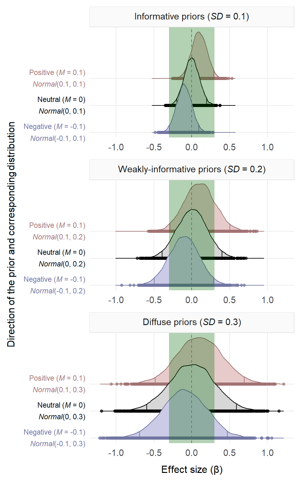
Priors used in the three studies. The green vertical rectangle shows the range of plausible effect sizes based on previous studies and on our frequentist analyses. In the informative priors, around 95% of the values fall within the range.
3. Prior predictive checks
The adequacy of each of these priors was assessed by performing prior predictive checks, in which we compared the observed data to the predictions of the model (Van de Schoot et al., 2021). Furthermore, in these checks we also tested the adequacy of two model-wide distributions: the traditional Gaussian distribution (default in most analyses) and an exponentially modified Gaussian—dubbed ‘ex-Gaussian’—distribution (Matzke & Wagenmakers, 2009). The ex-Gaussian distribution was considered because the residual errors of the frequentist models were not normally distributed (Lo & Andrews, 2015), and because this distribution was found to be more appropriate than the Gaussian one in a previous, related study (see supplementary materials of Rodríguez-Ferreiro et al., 2020). The ex-Gaussian distribution had an identity link function, which preserves the interpretability of the coefficients, as opposed to a transformation applied directly to the dependent variable (Lo & Andrews, 2015). The results of these prior predictive checks revealed that the priors were adequate, and that the ex-Gaussian distribution was more appropriate than the Gaussian one, converging with Rodríguez-Ferreiro et al. (2020). Therefore, the ex-Gaussian distribution was used in the final models.
Models with a Gaussian distribution
The figures below show the prior predictive checks for the Gaussian models. These plots show the maximum, mean and minimum values of the observed data (\(y\)) and those of the predicted distribution (\(y_{rep}\), which stands for replications of the outcome). The way of interpreting these plots is by comparing the observed data to the predicted distribution. The specifics of this comparison vary across the three plots. First, in the upper plot, which shows the maximum values, the ideal scenario would show the observed maximum value (\(y\)) overlapping with the maximum value of the predicted distribution (\(y_{rep}\)). Second, in the middle plot, showing the mean values, the ideal scenario would show the observed mean value (\(y\)) overlapping with the mean value of the predicted distribution (\(y_{rep}\)). Last, in the lower plot, which shows the minimum values, the ideal scenario would have the observed minimum value (\(y\)) overlapping with the minimum value of the predicted distribution (\(y_{rep}\)). While the overlap need not be absolute, the closer the observed and the predicted values are on the X axis, the better. As such, the three predictive checks below—corresponding to models that used the default Gaussian distribution—show that the priors fitted the data acceptably but not very well.
Models with an exponentially-modified Gaussian (i.e., ex-Gaussian) distribution
In contrast to the above results, the figures below demonstrate that, when an ex-Gaussian distribution was used, the priors fitted the data far better, which converged with the results of a similar comparison performed by Rodríguez-Ferreiro et al. (2020; see supplementary materials of the latter study).
4. Posterior predictive checks
Based on the results from the prior predictive checks, the ex-Gaussian distribution was used in the final models. Next, posterior predictive checks were performed to assess the consistency between the observed data and new data predicted by the posterior distributions (Van de Schoot et al., 2021). The figure below presents the posterior predictive checks for the latter models. The interpretation of these plots is simple: the distributions of the observed (\(y\)) and the predicted data (\(y_{rep}\)) should be as similar as possible. As such, the plots below suggest that the results are trustworthy.
5. Prior sensitivity analysis
In the main analysis, the informative, weakly-informative and diffuse priors were used in separate models. In other words, in each model, all priors had the same degree of informativeness (as done in Pregla et al., 2021; Rodríguez-Ferreiro et al., 2020; Stone et al., 2020; Stone et al., 2021). In this way, a prior sensitivity analysis was performed to acknowledge the likely influence of the priors on the posterior distributions—that is, on the results (Lee & Wagenmakers, 2014; Stone et al., 2020; Van de Schoot et al., 2021).
We’ll first load a custom function (frequentist_bayesian_plot) from GitHub.
source('https://raw.githubusercontent.com/pablobernabeu/language-sensorimotor-simulation-PhD-thesis/main/R_functions/frequentist_bayesian_plot.R')# Presenting the frequentist and the Bayesian estimates in the same plot.
# For this purpose, the frequentist results are merged into a plot from
# brms::mcmc_plot()
# install.packages('devtools')
# library(devtools)
# install_version('tidyverse', '1.3.1') # Due to breaking changes, Version 1.3.1 is required.
# install_version('ggplot2', '5.3.5') # Due to breaking changes, Version 5.3.5 is required.
library(tidyverse)
library(ggplot2)
library(Cairo)
# Load frequentist coefficients (estimates and confidence intervals)
KR_summary_semanticpriming_lmerTest =
readRDS(gzcon(url('https://github.com/pablobernabeu/language-sensorimotor-simulation-PhD-thesis/blob/main/semanticpriming/frequentist_analysis/results/KR_summary_semanticpriming_lmerTest.rds?raw=true')))
confint_semanticpriming_lmerTest =
readRDS(gzcon(url('https://github.com/pablobernabeu/language-sensorimotor-simulation-PhD-thesis/blob/main/semanticpriming/frequentist_analysis/results/confint_semanticpriming_lmerTest.rds?raw=true')))
# Below are the default names of the effects
# rownames(KR_summary_semanticpriming_lmerTest$coefficients)
# rownames(confint_semanticpriming_lmerTest)
# Load Bayesian posterior distributions
semanticpriming_posteriordistributions_informativepriors_exgaussian =
readRDS(gzcon(url('https://github.com/pablobernabeu/language-sensorimotor-simulation-PhD-thesis/blob/main/semanticpriming/bayesian_analysis/results/semanticpriming_posteriordistributions_informativepriors_exgaussian.rds?raw=true')))
semanticpriming_posteriordistributions_weaklyinformativepriors_exgaussian =
readRDS(gzcon(url('https://github.com/pablobernabeu/language-sensorimotor-simulation-PhD-thesis/blob/main/semanticpriming/bayesian_analysis/results/semanticpriming_posteriordistributions_weaklyinformativepriors_exgaussian.rds?raw=true')))
semanticpriming_posteriordistributions_diffusepriors_exgaussian =
readRDS(gzcon(url('https://github.com/pablobernabeu/language-sensorimotor-simulation-PhD-thesis/blob/main/semanticpriming/bayesian_analysis/results/semanticpriming_posteriordistributions_diffusepriors_exgaussian.rds?raw=true')))
# Below are the default names of the effects
# levels(semanticpriming_posteriordistributions_weaklyinformativepriors_exgaussian$data$parameter)
# Reorder the components of interactions in the frequentist results to match
# with the order present in the Bayesian results.
rownames(KR_summary_semanticpriming_lmerTest$coefficients) =
rownames(KR_summary_semanticpriming_lmerTest$coefficients) %>%
str_replace(pattern = 'z_recoded_interstimulus_interval:z_cosine_similarity',
replacement = 'z_cosine_similarity:z_recoded_interstimulus_interval') %>%
str_replace(pattern = 'z_recoded_interstimulus_interval:z_visual_rating_diff',
replacement = 'z_visual_rating_diff:z_recoded_interstimulus_interval')
rownames(confint_semanticpriming_lmerTest) =
rownames(confint_semanticpriming_lmerTest) %>%
str_replace(pattern = 'z_recoded_interstimulus_interval:z_cosine_similarity',
replacement = 'z_cosine_similarity:z_recoded_interstimulus_interval') %>%
str_replace(pattern = 'z_recoded_interstimulus_interval:z_visual_rating_diff',
replacement = 'z_visual_rating_diff:z_recoded_interstimulus_interval')
# Create a vector containing the names of the effects. This vector will be passed
# to the plotting function.
new_labels =
semanticpriming_posteriordistributions_weaklyinformativepriors_exgaussian$data$parameter %>%
unique %>%
# Remove the default 'b_' from the beginning of each effect
str_remove('^b_') %>%
# Put Intercept in parentheses
str_replace(pattern = 'Intercept', replacement = '(Intercept)') %>%
# First, adjust names of variables (both in main effects and in interactions)
str_replace(pattern = 'z_target_word_frequency',
replacement = 'Target-word frequency') %>%
str_replace(pattern = 'z_target_number_syllables',
replacement = 'Number of target-word syllables') %>%
str_replace(pattern = 'z_word_concreteness_diff',
replacement = 'Word-concreteness difference') %>%
str_replace(pattern = 'z_cosine_similarity',
replacement = 'Language-based similarity') %>%
str_replace(pattern = 'z_visual_rating_diff',
replacement = 'Visual-strength difference') %>%
str_replace(pattern = 'z_attentional_control',
replacement = 'Attentional control') %>%
str_replace(pattern = 'z_vocabulary_size',
replacement = 'Vocabulary size') %>%
str_replace(pattern = 'z_recoded_participant_gender',
replacement = 'Gender') %>%
str_replace(pattern = 'z_recoded_interstimulus_interval',
replacement = 'SOA') %>%
# Show acronym in main effect of SOA
str_replace(pattern = '^SOA$',
replacement = 'Stimulus onset asynchrony (SOA)') %>%
# Second, adjust order of effects in interactions. In the output from the model,
# the word-level variables of interest (i.e., 'z_cosine_similarity' and
# 'z_visual_rating_diff') sometimes appeared second in their interactions. For
# better consistency, the code below moves those word-level variables (with
# their new names) to the first position in their interactions. Note that the
# order does not affect the results in any way.
sub('(\\w+.*):(Language-based similarity|Visual-strength difference)',
'\\2:\\1',
.) %>%
# Replace colons denoting interactions with times symbols
str_replace(pattern = ':', replacement = ' × ')
# Create plots, beginning with the informative-prior model
plot_semanticpriming_frequentist_bayesian_plot_informativepriors_exgaussian =
frequentist_bayesian_plot(KR_summary_semanticpriming_lmerTest,
confint_semanticpriming_lmerTest,
semanticpriming_posteriordistributions_informativepriors_exgaussian,
labels = new_labels, interaction_symbol_x = TRUE,
vertical_line_at_x = 0, x_title = 'Effect size (β)',
x_axis_labels = 3, note_frequentist_no_prior = TRUE) +
ggtitle('Prior *SD* = 0.1')
#####
plot_semanticpriming_frequentist_bayesian_plot_weaklyinformativepriors_exgaussian =
frequentist_bayesian_plot(KR_summary_semanticpriming_lmerTest,
confint_semanticpriming_lmerTest,
semanticpriming_posteriordistributions_weaklyinformativepriors_exgaussian,
labels = new_labels, interaction_symbol_x = TRUE,
vertical_line_at_x = 0, x_title = 'Effect size (β)',
x_axis_labels = 3, note_frequentist_no_prior = TRUE) +
ggtitle('Prior *SD* = 0.2') +
theme(axis.text.y = element_blank())
#####
plot_semanticpriming_frequentist_bayesian_plot_diffusepriors_exgaussian =
frequentist_bayesian_plot(KR_summary_semanticpriming_lmerTest,
confint_semanticpriming_lmerTest,
semanticpriming_posteriordistributions_diffusepriors_exgaussian,
labels = new_labels, interaction_symbol_x = TRUE,
vertical_line_at_x = 0, x_title = 'Effect size (β)',
x_axis_labels = 3, note_frequentist_no_prior = TRUE) +
ggtitle('Prior *SD* = 0.3') +
theme(axis.text.y = element_blank())The figure below presents the posterior distribution of each effect in each model. The frequentist estimates are also shown to facilitate the comparison.
plot_semanticpriming_frequentist_bayesian_plot_informativepriors_exgaussian +
    plot_semanticpriming_frequentist_bayesian_plot_weaklyinformativepriors_exgaussian +
    plot_semanticpriming_frequentist_bayesian_plot_diffusepriors_exgaussian +

    plot_layout(ncol = 3, guides = 'collect') & theme(legend.position = 'bottom')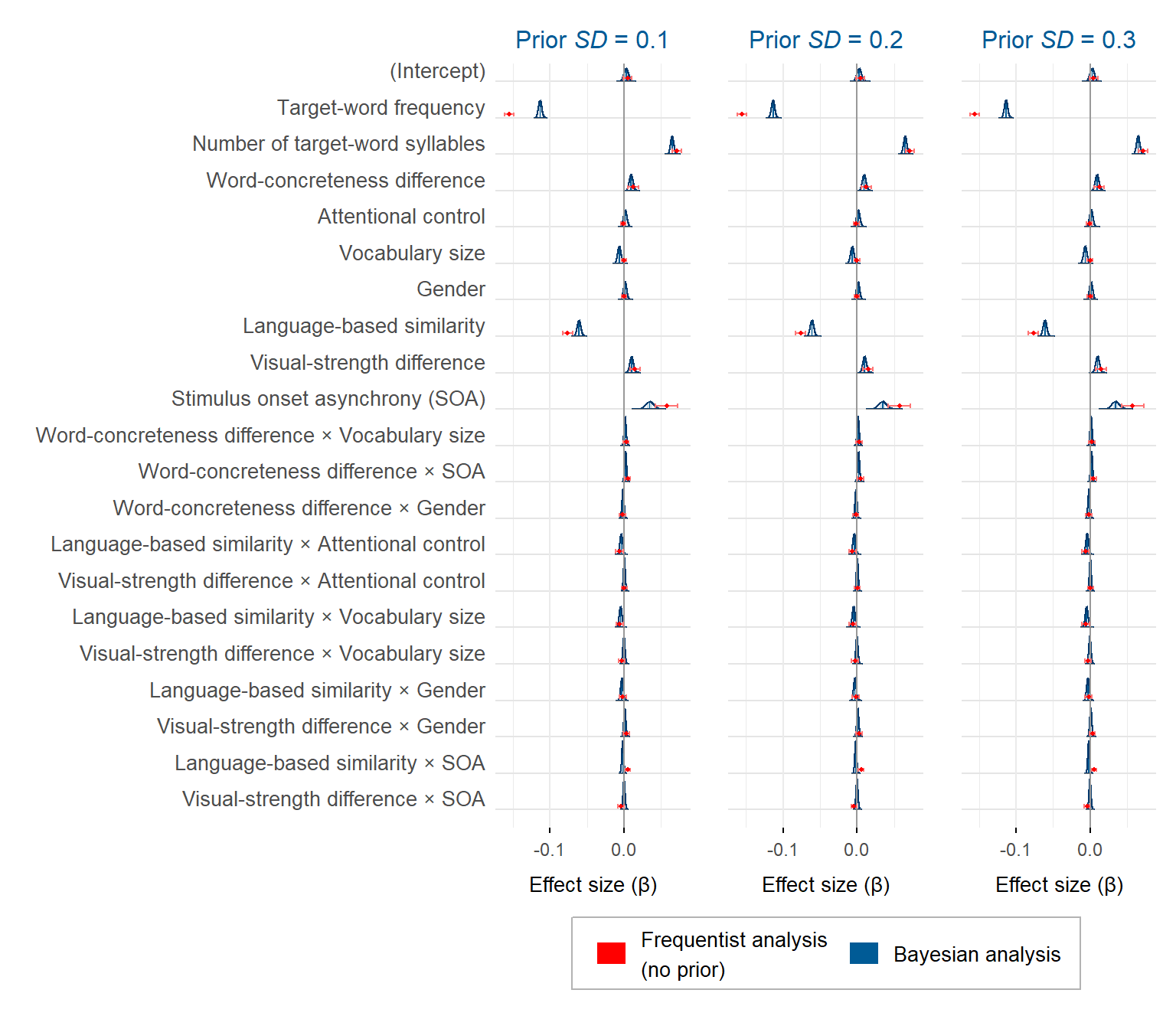
Estimates from the frequentist analysis (in red) and from the Bayesian analysis (in blue) for the semantic priming study, in each model. The frequentist means (represented by points) are flanked by 95% confidence intervals. The Bayesian means (represented by vertical lines) are flanked by 95% credible intervals in light blue (in some cases, the interval is occluded by the bar of the mean)
A blog post on the frequentist-Bayesian plots is also available.
Session info
If you encounter any blockers while reproduce the above analyses using the materials at https://osf.io/gt5uf, my current session info may be useful. For instance, the legend of the last plot may not show if the latest versions of the ggplot2 and the tidyverse packages are used. Instead, ggplot2 3.3.5 and tidyverse 1.3.1 should be installed using install_version('ggplot2', '3.3.5') and install_version('tidyverse', '1.3.1').
sessionInfo()## R version 4.2.3 (2023-03-15 ucrt)
## Platform: x86_64-w64-mingw32/x64 (64-bit)
## Running under: Windows 10 x64 (build 22621)
##
## Matrix products: default
##
## locale:
## [1] LC_COLLATE=English_United Kingdom.utf8
## [2] LC_CTYPE=English_United Kingdom.utf8
## [3] LC_MONETARY=English_United Kingdom.utf8
## [4] LC_NUMERIC=C
## [5] LC_TIME=English_United Kingdom.utf8
##
## attached base packages:
## [1] stats graphics grDevices utils datasets methods base
##
## other attached packages:
## [1] Cairo_1.6-0 forcats_1.0.0 stringr_1.5.0
## [4] purrr_1.0.1 readr_2.1.4 tidyr_1.3.0
## [7] tibble_3.2.1 tidyverse_1.3.1 papaja_0.1.1
## [10] tinylabels_0.2.3 patchwork_1.1.2 ggtext_0.1.2
## [13] ggridges_0.5.4 ggplot2_3.3.5 dplyr_1.1.1
## [16] knitr_1.42 xaringanExtra_0.7.0
##
## loaded via a namespace (and not attached):
## [1] fs_1.6.1 lubridate_1.9.2 insight_0.19.2 httr_1.4.6
## [5] tools_4.2.3 backports_1.4.1 bslib_0.4.2 utf8_1.2.3
## [9] R6_2.5.1 DBI_1.1.3 colorspace_2.1-0 withr_2.5.0
## [13] tidyselect_1.2.0 emmeans_1.8.7 compiler_4.2.3 cli_3.4.1
## [17] rvest_1.0.3 xml2_1.3.3 sandwich_3.0-2 labeling_0.4.2
## [21] bookdown_0.33.3 bayestestR_0.13.1 sass_0.4.6 scales_1.2.1
## [25] mvtnorm_1.1-3 commonmark_1.9.0 digest_0.6.31 rmarkdown_2.21
## [29] pkgconfig_2.0.3 htmltools_0.5.5 dbplyr_2.3.2 fastmap_1.1.1
## [33] highr_0.10 rlang_1.1.0 readxl_1.4.2 rstudioapi_0.14
## [37] jquerylib_0.1.4 farver_2.1.1 generics_0.1.3 zoo_1.8-11
## [41] jsonlite_1.8.4 magrittr_2.0.3 parameters_0.21.1 Matrix_1.6-1
## [45] Rcpp_1.0.10 munsell_0.5.0 fansi_1.0.4 lifecycle_1.0.3
## [49] stringi_1.7.12 multcomp_1.4-23 yaml_2.3.7 MASS_7.3-60
## [53] plyr_1.8.8 grid_4.2.3 crayon_1.5.2 lattice_0.21-8
## [57] haven_2.5.2 splines_4.2.3 gridtext_0.1.5 hms_1.1.3
## [61] pillar_1.9.0 uuid_1.1-0 markdown_1.5 estimability_1.4.1
## [65] effectsize_0.8.3 codetools_0.2-19 reprex_2.0.2 glue_1.6.2
## [69] evaluate_0.21 blogdown_1.16 modelr_0.1.11 vctrs_0.6.1
## [73] tzdb_0.4.0 cellranger_1.1.0 gtable_0.3.3 datawizard_0.8.0
## [77] cachem_1.0.7 xfun_0.38 xtable_1.8-4 broom_1.0.4
## [81] survival_3.5-7 timechange_0.2.0 TH.data_1.1-1