At Greg, 8 am
 Wikimedia Commmons (https://commons.wikimedia.org/wiki/File:Charmers_Cafe_on_a_quiet_morning.jpg)
The clock strikes a certain hour, below all the Greg’s teaspoons at play. Results o’clock. The usual, please.
Usual table. summaryby (having to get the first peek in the cafeteria can only add zest). summaryBy(RT ~ list(Ptp, Group, Cond), behdata, FUN=summary). So, hardly any of the 95% Confidence Intervals contain 0. Does this really mean…?
‘For example, the hypothesis of equality of population means will be rejected at the 0.05 level if and only if a 95% CI for the mean difference does not contain 0.’
— Dallal (2002; http://www.jerrydallal.com/lhsp/pval.htm)
Of course. The CI just has that and more. The window is showing a chilly 1999 morning. Let’s see the summary again. Wee standard deviations. By card, please.
Mmm, the air outside is worth gingering up…
The trials!
The assumption of independence spoils another morning.
This new data consisted of response times (RT) that had been collected over several trials. The single dependent variable, RT, was accompanied by other variables which could be analyzed as independent variables. These included Group, Trial Number, and a within-subjects Condition. What had to be done first off, in order to take the usual table? The trials!
Assumption of independence of observations
One must account for any redundant measures below the level of participants (the experimental trials, in this case), so that the sample size (N) used for any summary statistics match the number of participants (or the largest group, n). Why? This is a central assumption in statistics: observations must be independent. We can observe the independence assumption differently, depending on whether we’re summarizing data or performing statistical tests.
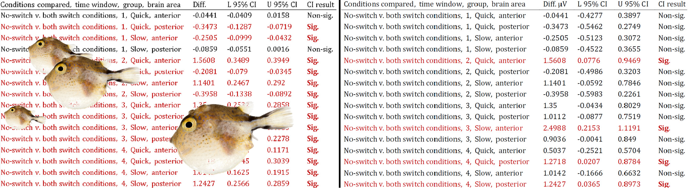
- For descriptive tables and plots (involving Standard Error/Deviation, Confidence Intervals, etc), the data ought to be aggregated to the level from which you want to generalize. That level is—in this case and very often—participants. Trials do not normally serve for statistical generalization (they’re good for experimental validity). This realization may come as a bummer if you have first seen the effect sizes in the un-aggregated data. The mirage (see red lines on the left table below) is caused by an inflated N (cf. red lines on the right-hand table). As an illustration, the tables below summarize data with an actual sample n = 23. However, the table on the right includes repeated measures that should have been aggregated, massively inflating n. The inflation of the sample size equals the product of all repeated measures that failed to be aggregated under participants.
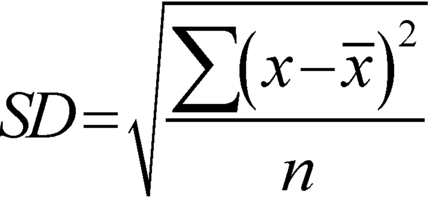
Measures of variance such as the Standard Deviation divide by the sample size. Thus, the larger the sample (N), the smaller the Standard Deviation, Standard Error, Confidence Interval…—that is, the variation or noise.
Aggregating is a snap. For example, with the aggregate() function in R, you just have to include all of your variables except that or those of the repeated measures:
behdata_aggreg = aggregate(behdata$RT, list(behdata$Ptp, behdata$Group, behdata$Cond),
data=behdata, FUN=mean)- In statistical tests, repeated measures below the participant level–e.g., trials–normally must be either factored in or aggregated. Barr and colleagues provide an easy, focused guide on this procedure. This is necessary because when the N in the analyses is augmented by unaccounted, redundant observations, the famous assumption of independence of observations is violated, and the results may be invalid, as Vasishth and Nicenboim (2016, p. 3) put it:
‘if we were to do a t-test on the unaggregated data, we would violate the independence assumption and the result of the t-test would be invalid.’
Now, usually the repetitions that concern us are the multiple trials or items in experiments, or other sub-participant measures. So what about participants–what are they never aggregated? McCarthy, Whittaker, Boyle, and Eyal (2017, p.10) note:
‘It has also been proposed that researchers aggregate the responses of participants within the same group and use the groups/clusters as the unit of analysis (Stevens, 2007). However, because this would result in losing sample size at the participant level, this approach is not optimal given the already small numbers of groups typically studied in group work research.’
Different procedure in linear mixed-effects models
Aggregation is no longer necessary, where linear mixed-effects models can be used. These models allow us to account for any clusters (Participants, Trials, Items…) by signing them into the error term (Brauer & Curtin, 2017).