Modality switch effects emerge early and increase throughout conceptual processing

How it works

Content

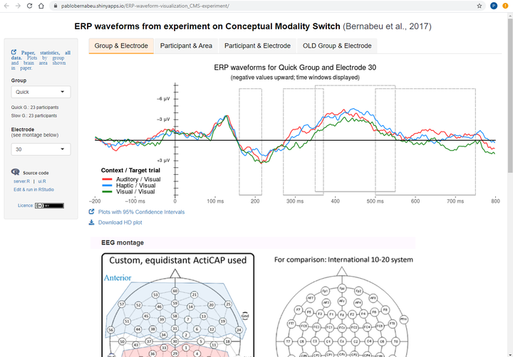
The data are from a psychology experiment on the comprehension of words, in which electroencephalographic (EEG) responses were measured. The data are presented in plots spanning 800 milliseconds (the duration of word processing). The aim of this Shiny app is to facilitate the exploration of the data by researchers and the public. Users can delve into the different sections of the data. In a hierarchical order, these sections are groups of participants, individual participants, brain areas, and electrodes.

Shiny apps in science

By creating this app, I tried to reach beyond the scope of current open science, which is often confined to files shared on data repositories. I believe that Shiny apps will become general practice in science within a few years ( see blog post or slides for more information).

Technical details

I used tabs on the upper area of the application page to avoid cramming the side bar with widgets. I adjusted the appearance of these tabs, and by means of 'reactivity' conditions, modified the inputs in the side bar depending on the active tab.

mainPanel(

	tags$style(HTML('
	    .tabbable > .nav > li > a                  		{background-color:white; color:#3E454E}
	    .tabbable > .nav > li > a:hover            		{background-color:#002555; color:white}
	    .tabbable > .nav > li[class=active] > a 		{background-color:#ECF4FF; color:black}
	    .tabbable > .nav > li[class=active] > a:hover	{background-color:#E7F1FF; color:black}
	')),

	tabsetPanel(id='tabvals',

            tabPanel(value=1, h4(strong('Group & Electrode')), br(), plotOutput('plot_GroupAndElectrode'),
			h5(a(strong('See plots with 95% Confidence Intervals'), href='https://osf.io/2tpxn/',
			target='_blank'), style='text-decoration: underline;'), 
			downloadButton('downloadPlot.1', 'Download HD plot'), br(), br(),
			# EEG montage
			img(src='https://preview.ibb.co/n7qiYR/EEG_montage.png', height=500, width=1000)),

            tabPanel(value=2, h4(strong('Participant & Area')), br(), plotOutput('plot_ParticipantAndLocation'),
			h5(a(strong('See plots with 95% Confidence Intervals'), href='https://osf.io/86ch9/',
			target='_blank'), style='text-decoration: underline;'), 
			downloadButton('downloadPlot.2', 'Download HD plot'), br(), br(),
			# EEG montage
			img(src='https://preview.ibb.co/n7qiYR/EEG_montage.png', height=500, width=1000)),

            tabPanel(value=3, h4(strong('Participant & Electrode')), br(), plotOutput('plot_ParticipantAndElectrode'),
			br(), downloadButton('downloadPlot.3', 'Download HD plot'), br(), br(),
			# EEG montage
			img(src='https://preview.ibb.co/n7qiYR/EEG_montage.png', height=500, width=1000)),

            tabPanel(value=4, h4(strong('OLD Group & Electrode')), br(), plotOutput('plot_OLDGroupAndElectrode'),
			h5(a(strong('See plots with 95% Confidence Intervals'), href='https://osf.io/dvs2z/',
			target='_blank'), style='text-decoration: underline;'), 
			downloadButton('downloadPlot.4', 'Download HD plot'), br(), br(),
			# EEG montage
			img(src='https://preview.ibb.co/n7qiYR/EEG_montage.png', height=500, width=1000))
	),

The data set was fairly large, considering the fact that it's hosted with the free plan. In order to lighten the processing, I split the data into various files, reducing the total size. Furthermore, I outsourced a particularly heavy set of plots (those with Confidence Intervals) to PDF files, to which I linked in the app.

h5(a(strong('See plots with 95% Confidence Intervals'), href='https://osf.io/dvs2z/',
			target='_blank'), style='text-decoration: underline;'),

I also used web links to the published paper and raw data, as well as to the server and ui scripts. These files, along with the data, are publicly available in this repository; they may be accessed within the "Files" section, by opening the folders "ERPs" -> "Analyses of ERPs averaged across trials" -> "Shiny app".

Another feature I added was the download button.

# From server.R script

spec_title = paste0('ERP waveforms for ', input$var.Group, ' Group, Electrode ', input$var.Electrodes.1, ' (negative values upward; time windows displayed)')

plot_GroupAndElectrode = ggplot(df2, aes(x=time, y=-microvolts, color=condition)) +
  geom_rect(xmin=160, xmax=216, ymin=7.5, ymax=-8, color = 'grey75', fill='black', alpha=0, linetype='longdash') +
  geom_rect(xmin=270, xmax=370, ymin=7.5, ymax=-8, color = 'grey75', fill='black', alpha=0, linetype='longdash') +
  geom_rect(xmin=350, xmax=550, ymin=8, ymax=-7.5, color = 'grey75', fill='black', alpha=0, linetype='longdash') +
  geom_rect(xmin=500, xmax=750, ymin=7.5, ymax=-8, color = 'grey75', fill='black', alpha=0, linetype='longdash') +
  geom_line(size=1, alpha = 1) + scale_linetype_manual(values=colours) +
  scale_y_continuous(limits=c(-8.38, 8.3), breaks=seq(-8,8,by=1), expand = c(0,0.1)) +
  scale_x_continuous(limits=c(-208,808),breaks=seq(-200,800,by=100), expand = c(0.005,0), labels= c('-200','-100 ms','0','100 ms','200','300 ms','400','500 ms','600','700 ms','800')) +
  ggtitle(spec_title) + theme_bw() + geom_vline(xintercept=0) +
  annotate(geom='segment', y=seq(-8,8,1), yend=seq(-8,8,1), x=-4, xend=8, color='black') +
  annotate(geom='segment', y=-8.2, yend=-8.38, x=seq(-200,800,100), xend=seq(-200,800,100), color='black') +
  geom_segment(x = -200, y = 0, xend = 800, yend = 0, size=0.5, color='black') +
  theme(legend.position = c(0.100, 0.150), legend.background = element_rect(fill='#EEEEEE', size=0),
	axis.title=element_blank(), legend.key.width = unit(1.2,'cm'), legend.text=element_text(size=17),
	legend.title = element_text(size=17, face='bold'), plot.title= element_text(size=20, hjust = 0.5, vjust=2),
	axis.text.y = element_blank(), axis.text.x = element_text(size = 14, vjust= 2.12, face='bold', color = 'grey32', family='sans'),
	axis.ticks=element_blank(), panel.border = element_blank(), panel.grid.major = element_blank(), 
	panel.grid.minor = element_blank(), plot.margin = unit(c(0.1,0.1,0,0), 'cm')) +
  annotate('segment', x=160, xend=216, y=-8, yend=-8, colour = 'grey75', size = 1.5) +
  annotate('segment', x=270, xend=370, y=-8, yend=-8, colour = 'grey75', size = 1.5) +
  annotate('segment', x=350, xend=550, y=-7.5, yend=-7.5, colour = 'grey75', size = 1.5) +
  annotate('segment', x=500, xend=750, y=-8, yend=-8, colour = 'grey75', size = 1.5) +
  scale_fill_manual(name = 'Context / Target trial', values=colours) +
  scale_color_manual(name = 'Context / Target trial', values=colours) +
  guides(linetype=guide_legend(override.aes = list(size=1.2))) +
   guides(color=guide_legend(override.aes = list(size=2.5))) +
# Print y axis labels within plot area:
  annotate('text', label = expression(bold('\u2013' * '3 ' * '\u03bc' * 'V')), x = -29, y = 3, size = 4.5, color = 'grey32', family='sans') +
  annotate('text', label = expression(bold('+3 ' * '\u03bc' * 'V')), x = -29, y = -3, size = 4.5, color = 'grey32', family='sans') +
  annotate('text', label = expression(bold('\u2013' * '6 ' * '\u03bc' * 'V')), x = -29, y = 6, size = 4.5, color = 'grey32', family='sans')

print(plot_GroupAndElectrode)

output$downloadPlot.1 <- downloadHandler(
	filename <- function(file){
	paste0(input$var.Group, ' group, electrode ', input$var.Electrodes.1, ', ', Sys.Date(), '.png')},
   	content <- function(file){
      		png(file, units='in', width=13, height=5, res=900)
      		print(plot_GroupAndElectrode)
      		dev.off()},
	contentType = 'image/png')
  } )

# From ui.R script

downloadButton('downloadPlot.1', 'Download HD plot')

Rising to the challenge

My experience with R Shiny has been so good I've been sharing it. Yet, on my first crawling days, I spent an eternity stuck with this elephant in my room: "μ". This μ letter (micro-souvenir from hell, as I later knew it), was part of the labels of my plots. All I knew was that I could not deploy the app online, even while I could perfectly launch it locally in my laptop. So, I wondered what use it was to deploy locally if I couldn't publish the app?! Eventually, I read about UTF-8 encoding in one forum. Bless them forums. All I had to do was use "Âμ" instead of the single "μ". A better option I found later was: expression("\u03bc").

Beyond encoding issues, I had a tough time embedding images. You know, the 'www' folder... To be honest, I still haven't handled the 'www' way--but where there's a will, there's a way. I managed to include my images by uploading them to a website and then entering their URL in "img(src", avoiding the use of folder paths.

img(src="https://preview.ibb.co/n7qiYR/EEG_montage.png 1", height=500, width=1000)

Long after I had built the app, I added another image--the favicon (the little icon on the browser tab).

tags$head(tags$link(rel="shortcut icon", href="https://image.ibb.co/fXUwzb/favic.png")),  # web favicon

Reference

Bernabeu, P., Willems, R. M., & Louwerse, M. M. (2017). Modality switch effects emerge early and increase throughout conceptual processing: Evidence from ERPs [Web application]. Retrieved from https://pablobernabeu.shinyapps.io/ERP-waveform-visualization_CMS-experiment