pilotr: Pilot the study before running it
Power calculations can feel reassuringly final. Choose an effect, enter a sample size and read off a percentage. That simplicity disappears in experiments where participants respond to many items. Participants and items both vary, their responses are crossed, and the model usually needs random slopes as well as random intercepts. The design has become too structured for a single formula.
I built pilotr to make those assumptions visible before data collection. It stores a proposed study as a portable specification, simulates the observations implied by it and fits the planned analysis repeatedly. The R and Python packages read the same specification and generate the same data from the same seed. Here I use it on a semantic-priming study with 30 participants and 24 items, to show what a design analysis has to weigh besides power.
A study that does not exist yet
The imagined experiment is a lexical-decision task. Every participant sees every target word after related and unrelated primes. Reaction times follow a shifted lognormal distribution, and the model includes item frequency, participant vocabulary and an interaction between vocabulary and priming.
The assumptions are deliberately concrete:
| Part of the design | Assumption |
|---|---|
| Participants | 30 |
| Items | 24 |
| Priming effect | 0.05 on the log scale, about 20 ms |
| Participant variation | Random intercept and priming slope |
| Item variation | Random intercept and priming slope |
| Response | Shifted lognormal reaction time |
The specification determines the analysis formula as well as the data generator. That prevents a quiet mismatch between the design used for power and the model eventually fitted.
model_formula(spec)#> .y ~ prime + z_freq + z_vocab + prime_z_vocab + (1 + prime |
#> subject) + (1 + prime | item)Looking at the imagined data
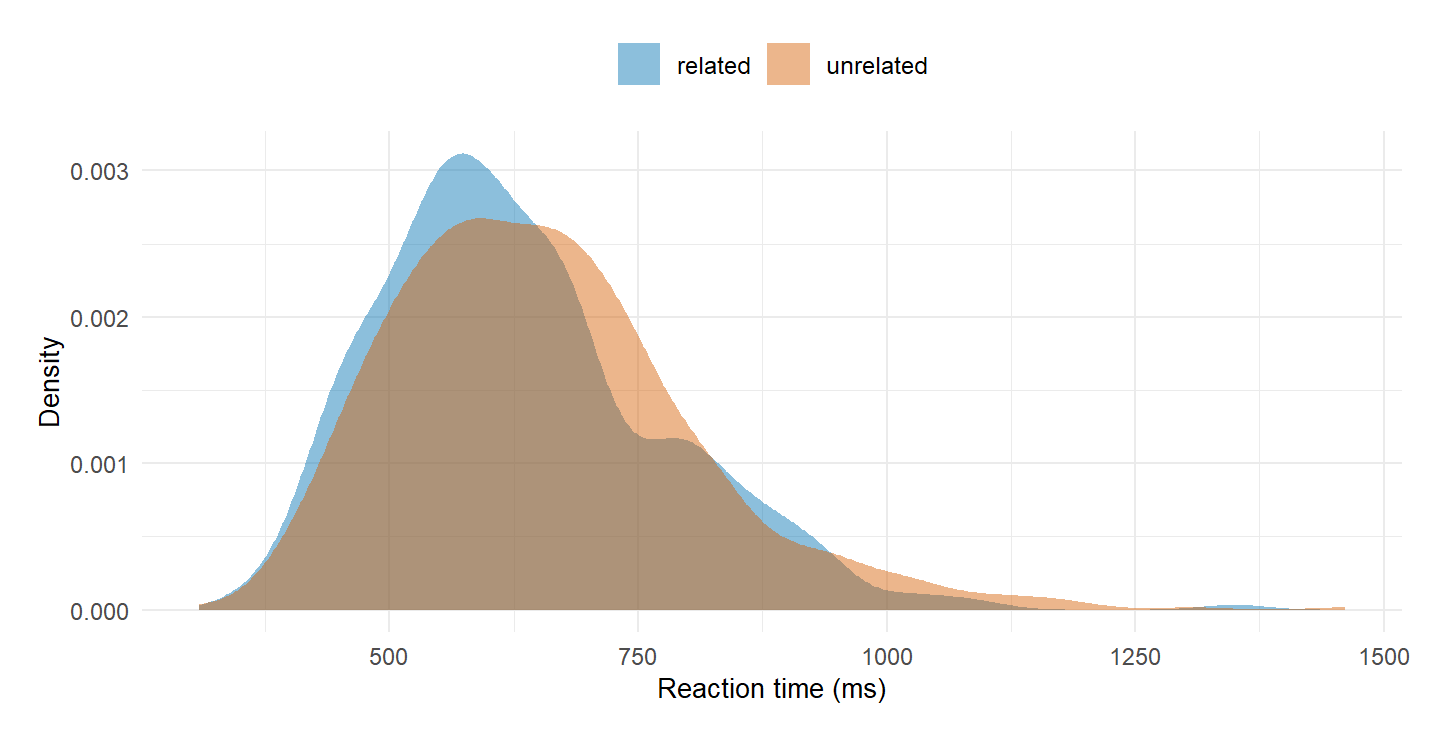
A single simulated data set is useful before any power calculation (DeBruine & Barr, 2021). It shows whether the assumptions produce recognisable observations. Here the reaction times are right-skewed, as intended, and unrelated primes shift the distribution slightly to the right.
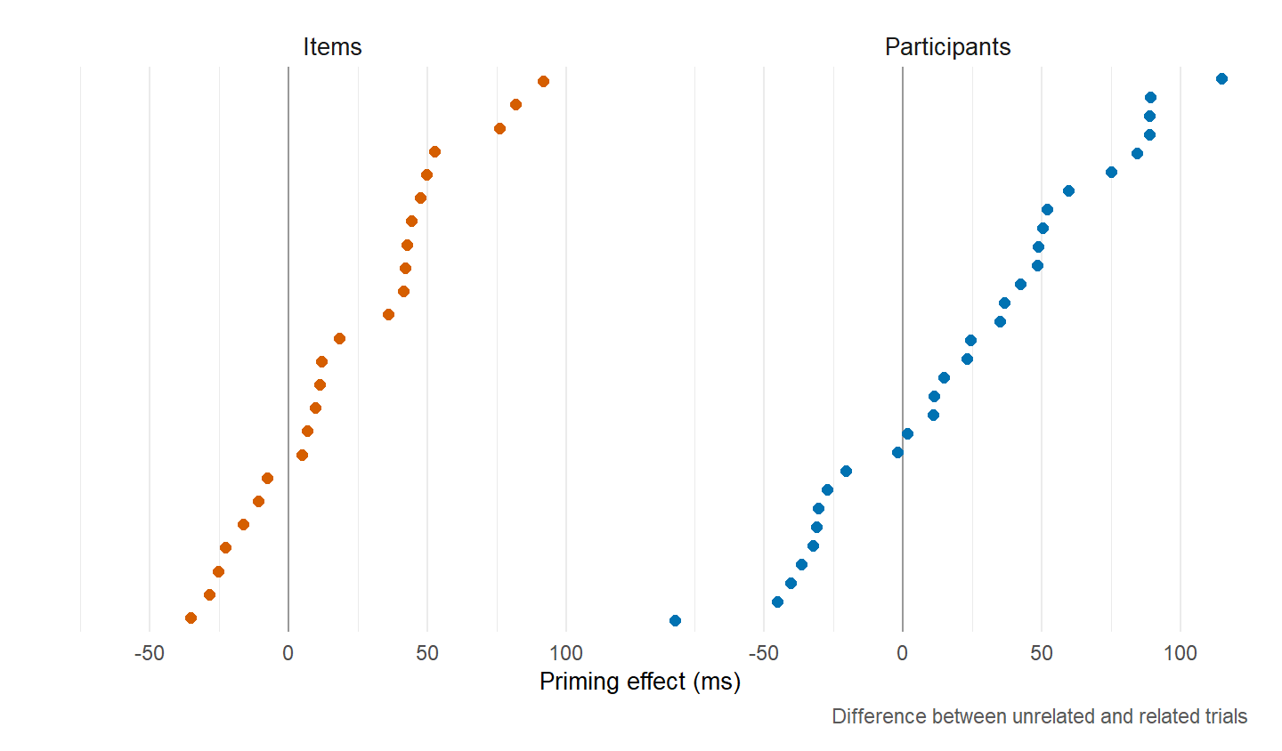
The average priming effect is only part of the picture. Because the specification gives participants and items their own priming slopes, some show a much larger difference than others, and in about a third of each set the difference runs the other way.
Detection is not estimation
The first design analysis repeatedly simulates the study and fits its mixed model. It records conventional power and singular fits. It also reports Type S error, the chance that a significant estimate has the wrong sign, and Type M error, the factor by which significant estimates exaggerate the true effect (Gelman & Carlin, 2014). To keep this article executable during a site build, the run below uses twelve replicates.
power_at_plan <- power_mixed(spec, n_sims = n_sims, workers = workers)
power_at_plan
#> Simulation-based power over 12 replicates (alpha = 0.05)
#> fits: 12 attempted, 12 returned, 6 converged cleanly, 6 singular, 6 with warnings
#> note: many fits were boundary-singular, so this model is richer than the design supports
#> effect true power mcse ci95 n_sig type_s type_m
#> prime 0.05 0.667 0.136 [0.391, 0.862] 8 0 1.039
#> z_freq -0.03 0.250 0.125 [0.089, 0.532] 3 0 1.648
#> z_vocab -0.02 0.000 0.000 [0.000, 0.242] 0 NA NA
#> prime_z_vocab 0.02 0.167 0.108 [0.047, 0.448] 2 0 2.016Twelve replicates are enough to prove the pipeline runs and nowhere near enough to pin down the estimate, since one simulated success moves the figure by more than eight percentage points. Everything below therefore shows the shape of each diagnostic and the quantity to read from it, and a planning run would repeat the same code a few hundred times, until its Monte Carlo error was acceptably small.
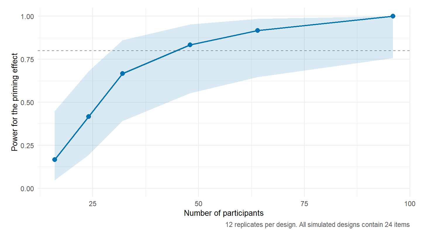
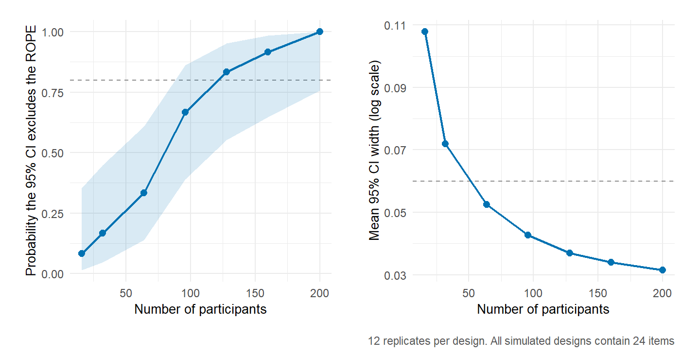
Power asks whether an effect would clear a threshold. I also want to know whether its interval would exclude effects too small to matter. With a region of practical equivalence (ROPE; Kruschke, 2018) of plus or minus 0.02 on the log scale, roughly 8 ms here, precision becomes a separate design criterion.
The significant estimates are the misleading ones
A low-powered study misses real effects, and it also distorts the ones it finds. Only unusually large estimates pass the significance threshold, so significance selects for exaggeration. To see that selection directly, I varied both the true effect and the number of participants.
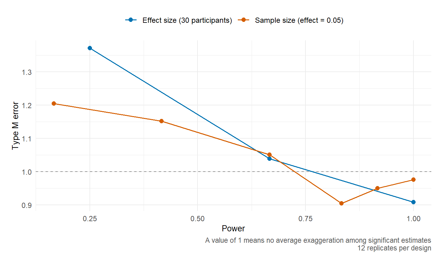
This run shows what a defensible planning run must examine together: detection, precision, magnitude error and singular fits. The warnings here would prompt me to increase the simulation count and reconsider the random-effects structure before recruiting a participant. Keeping that structure maximal protects the Type I error rate (Barr et al., 2013), and trimming it when the data cannot support it protects power (Matuschek et al., 2017). A planning run is where that trade-off can be examined instead of assumed. That ability to expose a design’s weak points is the useful result of the exercise.
The complete specification format, response families, mixed-model options and browser interface are in the R documentation, Python documentation and no-code app.
References
Barr, D. J., Levy, R., Scheepers, C., & Tily, H. J. (2013). Random effects structure for confirmatory hypothesis testing: Keep it maximal. Journal of Memory and Language, 68(3), 255–278. https://doi.org/10.1016/j.jml.2012.11.001
DeBruine, L. M., & Barr, D. J. (2021). Understanding mixed-effects models through data simulation. Advances in Methods and Practices in Psychological Science, 4(1). https://doi.org/10.1177/2515245920965119
Gelman, A., & Carlin, J. (2014). Beyond power calculations: Assessing Type S (sign) and Type M (magnitude) errors. Perspectives on Psychological Science, 9(6), 641–651. https://doi.org/10.1177/1745691614551642
Kruschke, J. K. (2018). Rejecting or accepting parameter values in Bayesian estimation. Advances in Methods and Practices in Psychological Science, 1(2), 270–280. https://doi.org/10.1177/2515245918771304
Matuschek, H., Kliegl, R., Vasishth, S., Baayen, H., & Bates, D. (2017). Balancing Type I error and power in linear mixed models. Journal of Memory and Language, 94, 305–315. https://doi.org/10.1016/j.jml.2017.01.001
Comments are provided by Disqus and are not loaded automatically. Loading them connects your browser to Disqus, which may use cookies and process data under its privacy policy. See this site's privacy notice for details.