lexsync: From a word-frequency corpus to an EEG-ready experiment

Put the design in data

The design below asks for 40 words in each frequency condition. Length, neighbourhood density and OLD20 are controls. The two lists will also be balanced on those controls and on frequency. Zipf frequency follows van Heuven et al. (2014), while OLD20 measures orthographic similarity as the mean edit distance from a word’s 20 nearest neighbours (Yarkoni et al., 2008).

design <- list(
  name = 'frequency_eeg',
  language = 'english',
  n_per_condition = 40,
  pool_filters = list(length = c(3, 7), frequency = c(3.8, 7.0)),
  conditions = list(
    list(name = 'high_frequency', define_by = list(frequency = c(5.2, 7.0))),
    list(name = 'low_frequency', define_by = list(frequency = c(3.8, 4.4)))
  ),
  match_on = c('length', 'n_density', 'old20'),
  counterbalance = list(
    lists = 2,
    optimise = TRUE,
    balance_on = c('length', 'n_density', 'old20', 'frequency')
  )
)

pool <- build_pool(lexicon, design$pool_filters)
candidate_counts <- vapply(
  design$conditions,
  function(condition) nrow(build_pool(pool, condition$define_by)),
  integer(1)
)
names(candidate_counts) <- vapply(design$conditions, `[[`, character(1), 'name')
candidate_counts

#> high_frequency  low_frequency 
#>             71            480

The high-frequency band is the smaller candidate set, so it limits the number and quality of possible matches. Keeping that count beside the design makes a shortfall interpretable instead of leaving it to appear as a mysterious matching failure.

Select and check the words

match_stimuli() spreads anchor words across the smaller frequency band and finds nearby words from the other condition in the standardised space of the control variables.

stimuli <- match_stimuli(pool, design, schema)
head(stimuli[, c('set', 'condition', 'word', 'frequency', 'length',
                  'n_density', 'old20')])

#>   set      condition    word frequency length n_density old20
#> 1   1 high_frequency    knew      5.20      4         3  1.75
#> 2   2 high_frequency    date      5.22      4        17  1.00
#> 3   3 high_frequency  energy      5.23      6         0  2.60
#> 4   4 high_frequency  points      5.23      6         5  1.65
#> 5   5 high_frequency running      5.23      7         3  1.80
#> 6   6 high_frequency    term      5.23      4         4  1.65

The report treats matching as an equivalence claim. For each control, it gives Cohen’s \(d\) with a 90% confidence interval and tests that interval against the design’s bound of half a standard deviation (Lakens, 2017). The frequency row describes the intended manipulation and is omitted from the figure.

report <- match_report(
  stimuli,
  c('frequency', 'length', 'n_density', 'old20'),
  schema
)
report$comparisons

#>       condition      reference dimension cohens_d d_ci_low d_ci_high var_ratio tost_p
#> 1 low_frequency high_frequency frequency    5.642    5.270     6.014     0.293 1.0000
#> 2 low_frequency high_frequency    length    0.000   -0.372     0.372     1.000 0.0141
#> 3 low_frequency high_frequency n_density    0.076   -0.296     0.448     0.632 0.0308
#> 4 low_frequency high_frequency     old20    0.016   -0.356     0.389     0.843 0.0168
#>   equivalent
#> 1      FALSE
#> 2       TRUE
#> 3       TRUE
#> 4       TRUE

controls <- subset(report$comparisons, dimension != 'frequency')
controls$dimension <- factor(
  controls$dimension,
  levels = rev(c('length', 'n_density', 'old20')),
  labels = rev(c('Word length', 'Neighbourhood density', 'OLD20'))
)

ggplot(controls, aes(cohens_d, dimension)) +
  annotate('rect', xmin = -0.5, xmax = 0.5, ymin = -Inf, ymax = Inf,
           fill = '#E8F1F5') +
  geom_vline(xintercept = 0, colour = '#66747B', linewidth = 0.5) +
  geom_pointrange(aes(xmin = d_ci_low, xmax = d_ci_high),
                  colour = '#006D77', linewidth = 0.7) +
  scale_x_continuous(limits = c(-0.65, 0.65), breaks = c(-0.5, 0, 0.5)) +
  labs(x = 'Standardised difference (low minus high), 90% CI', y = NULL,
       title = 'Realised balance on the control variables',
       subtitle = 'Shading marks the prespecified equivalence region') +
  theme_minimal(base_size = 11) +
  theme(panel.grid.major.y = element_blank(),
        plot.title.position = 'plot',
        plot.title = element_text(size = 11, face = 'bold'),
        plot.subtitle = element_text(size = 10),
        axis.title = element_text(size = 10),
        axis.text = element_text(size = 9))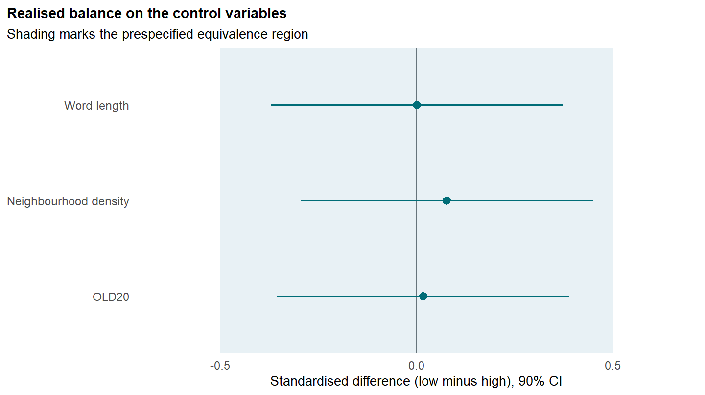

The point estimates are useful, but the intervals carry the uncertainty. With only a few items, near-zero estimates can still be too imprecise to support an equivalence claim.

Carry the items into the experiment

The design also describes a trial. A fixation is followed by the word, an onset-locked condition trigger, a response window and a jittered blank interval. Jitter is derived from a keyed hash of the design and seed, so rebuilding the experiment preserves the realised timing.

design$events <- list(
  list(type = 'fixation', content = '+', duration_ms = 500),
  list(type = 'text', content = '{word}', duration_ms = 800,
       trigger = 'condition', onset_locked = TRUE),
  list(type = 'response', keys = c('f', 'j'), timeout_ms = 2000),
  list(type = 'blank', duration = list(jitter = c(400, 800), as = 'iti_ms'))
)

list_plan <- balance_lists(stimuli, design, schema)
trials <- counterbalance(stimuli, design, schema, list_plan$list_of_set)
trials <- resolve_trial_timing(trials, design, schema)
trials <- assign_triggers(trials)

c(cost_before = list_plan$report$cost_before,
  cost_after = list_plan$report$cost_after,
  swaps = list_plan$report$n_swaps)

#> cost_before  cost_after       swaps 
#>      743080       17880           5

head(trials[, c('list', 'trial', 'condition', 'word', 'iti_ms',
                'condition_trigger')])

#>   list trial      condition    word iti_ms condition_trigger
#> 1    1     1  low_frequency approve    696               101
#> 2    1     2 high_frequency    knew    504               102
#> 3    1     3 high_frequency  mother    643               102
#> 4    1     4  low_frequency    loop    688               101
#> 5    1     5 high_frequency    lost    489               102
#> 6    1     6  low_frequency   ghana    498               101

The exported files all read from this trial table. In the PsychoPy script, win.callOnFlip sends the trigger on the refresh that presents the word.

experiments <- export_experiments(trials, design, schema, output_dir)
basename(unlist(experiments))

#> [1] "frequency_eeg_english_psychopy.py" "frequency_eeg_english.osexp"      
#> [3] "frequency_eeg_english.html"

psychopy_code <- readLines(experiments$psychopy, warn = FALSE)
grep('^\\s*(TRIGGER_HOLD_MS\\s*=|win\\.callOnFlip\\()', psychopy_code,
     value = TRUE, perl = TRUE)

#> [1] "TRIGGER_HOLD_MS = 50"                                 
#> [2] "        win.callOnFlip(port.setData, trigger)"        
#> [3] "            win.callOnFlip(port.setData, 0)"          
#> [4] "                win.callOnFlip(port.setData, trig)"   
#> [5] "    win.callOnFlip(port.setData, BLOCK_START_TRIGGER)"
#> [6] "    win.callOnFlip(port.setData, BLOCK_END_TRIGGER)"

Limits

Matching can only use what the candidate corpus contains. The bundled lexicon is suitable for this demonstration, but it includes proper nouns, estimates syllables from spelling and has no part-of-speech information. A study should therefore supply its own exclusions and any norms needed for the research question. Equivalence also depends on the bound chosen before selection. The default half-standard-deviation region is not a universal definition of an acceptable match.

The R documentation and Python documentation cover pseudoword generation, semantic norms, continuous designs, Latin-square counterbalancing and the full file-based pipeline. The useful boundary is simple: the design records the intended experiment, while the generated tables and reports record what was realised.

References

Lakens, D. (2017). Equivalence tests: A practical primer for t tests, correlations, and meta-analyses. Social Psychological and Personality Science, 8(4), 355–362. https://doi.org/10.1177/1948550617697177
van Heuven, W. J. B., Mandera, P., Keuleers, E., & Brysbaert, M. (2014). SUBTLEX-UK: A new and improved word frequency database for British English. Quarterly Journal of Experimental Psychology, 67(6), 1176–1190. https://doi.org/10.1080/17470218.2013.850521
Yarkoni, T., Balota, D., & Yap, M. (2008). Moving beyond Coltheart’s N: A new measure of orthographic similarity. Psychonomic Bulletin & Review, 15(5), 971–979. https://doi.org/10.3758/PBR.15.5.971
Comments are provided by Disqus and are not loaded automatically. Loading them connects your browser to Disqus, which may use cookies and process data under its privacy policy. See this site's privacy notice for details.