depictr: One visual language from first look to final figure
The figures in an analysis are rarely made all at once. An exploratory density plot may survive into a talk, a model adds a forest plot and a reviewer asks for a diagnostic or a Bayesian comparison. When each stage uses different defaults, one analysis acquires several palettes, type sizes and conventions. Accessibility is then checked, if at all, after the visual decisions have already spread through the project.
I wrote depictr to give those stages a shared visual language. It provides plotting functions for common statistical objects, but each function returns an ordinary ggplot2 object that can still be changed. It also measures the finished figure against explicit checks for contrast, text size and reliance on colour. The same conventions are available in the R package and the Python package.
The example data come from a lexical-decision experiment bundled with the package. Participants responded to words preceded by semantically related or unrelated primes, presented visually or auditorily.
library(depictr)
library(ggplot2)
packageVersion('depictr')
#> [1] '0.3.0'data('lexical_decision', package = 'depictr')
correct <- subset(lexical_decision, accuracy == 1)
c(participants = length(unique(lexical_decision$participant)),
items = length(unique(lexical_decision$item)),
trials = nrow(lexical_decision))#> participants items trials
#> 24 40 960Begin with the observed distribution
Reaction times are skewed, so a mean and standard deviation do not show the whole pattern. An empirical cumulative distribution avoids a choice of bins and makes the quartiles directly visible.
ecdf_plot(
  lexical_decision,
  RT,
  group = condition,
  reference_quantiles = c(0.25, 0.5, 0.75),
  legend_inside = TRUE,
  title = 'Related primes are faster across the distribution'
) +
  labs(x = 'Reaction time (ms)', colour = NULL)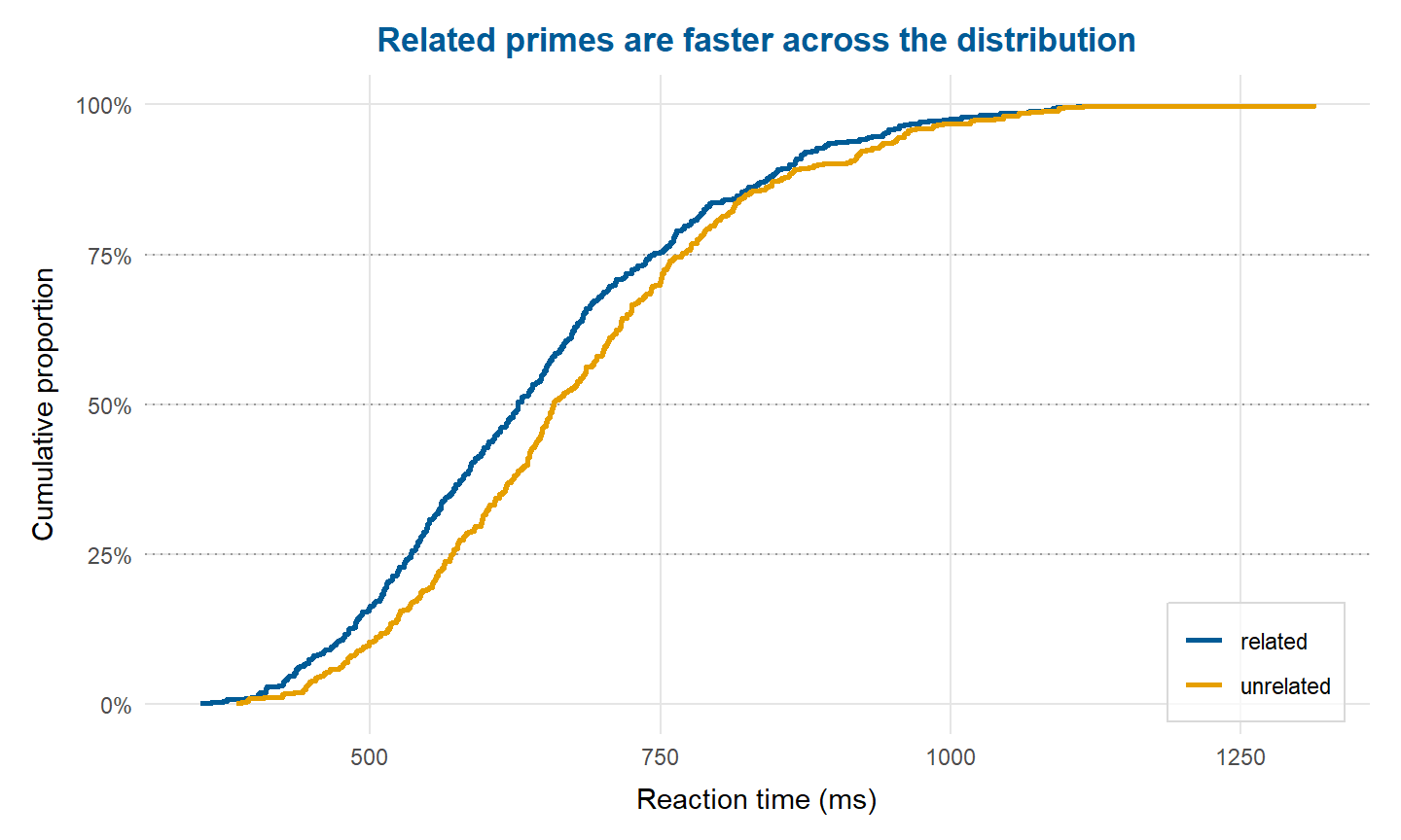
The separation is not confined to a handful of slow responses. Related trials remain shifted towards shorter reaction times through much of the distribution, which gives the later model result a visible empirical context.
Keep the same language for the model
The model includes priming condition, presentation modality and word frequency, with crossed random intercepts for participants and items. coefficient_plot() reads the fitted object directly and places the fixed effects on a common standardised scale.
fit <- lmerTest::lmer(
  RT ~ condition + modality + word_frequency +
    (1 | participant) + (1 | item),
  data = correct
)

term_labels <- c(
  conditionunrelated = 'Unrelated priming',
  modalityauditory = 'Auditory modality',
  word_frequency = 'Word frequency (Zipf)'
)

tidy_estimates(fit)
#> term estimate std.error conf.low conf.high
#> 1 (Intercept) 708.01334 27.253962 654.596553 761.43012
#> 2 conditionunrelated 31.95745 8.119043 16.044418 47.87048
#> 3 modalityauditory 25.34713 8.123180 9.425993 41.26827
#> 4 word_frequency -21.89472 5.860301 -33.380696 -10.40874coefficient_plot(
fit,
standardise = TRUE,
order = 'ascending',
labels = term_labels,
title = 'Estimated effects on reaction time',
x_lab = 'Change in reaction time (ms) per SD of predictor'
)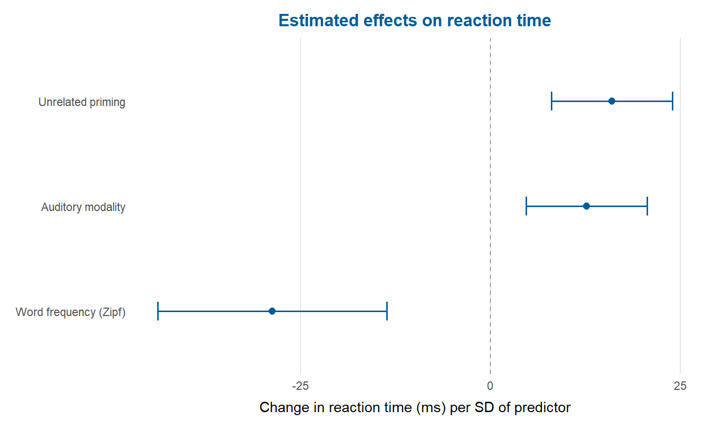
This continuity keeps the colour, typography and interval conventions stable as the analysis moves from observations to estimates, so the reader can concentrate on the result.
Audit the figure that will be published
A colourblind-safe palette does not guarantee an accessible figure. Contrast against the background and the use of a second visual channel depend on the particular plot. The package therefore audits a built plot, not only its palette.
first_draft <- explore_distribution(
  lexical_decision,
  RT,
  group = condition,
  type = 'density',
  legend_inside = TRUE,
  title = 'Lexical-decision time by priming condition'
)
check_figure(first_draft)
#> check measured threshold verdict
#> 1 colour_separability 119.21 5.0 pass
#> 2 colour_separability_protan 108.92 5.0 pass
#> 3 colour_separability_deutan 121.29 5.0 pass
#> 4 colour_separability_tritan 77.90 5.0 pass
#> 5 greyscale_separability 33.34 5.0 pass
#> 6 text_size 8.80 6.0 pass
#> 7 text_contrast 7.15 4.5 pass
#> 8 geometry_contrast 2.25 3.0 fail
#> 9 redundant_encoding 0.00 1.0 fail
#> detail
#> 1 Closest pair #005b96 and #e69f00 of 2 encoding colours.
#> 2 Closest pair #005b96 and #e69f00 of 2 encoding colours.
#> 3 Closest pair #005b96 and #e69f00 of 2 encoding colours.
#> 4 Closest pair #005b96 and #e69f00 of 2 encoding colours.
#> 5 Closest pair #005b96 and #e69f00 in CIE lightness.
#> 6 Smallest text 8.80 pt, drawn at 17.78 cm and printed at 17.78 cm.
#> 7 Lowest-contrast text #005b96 on #ffffff.
#> 8 Lowest-contrast colour #e69f00 on #ffffff.
#> 9 Colour alone distinguishes the groups.The default density fails two checks. Its orange fill falls below the package’s contrast threshold against white, and colour is the only channel separating the conditions. The corrected density plot uses a darker vermilion and adds line type. Those changes address the measured failures without changing the data or the statistical display.
final_figure <- explore_distribution(
  lexical_decision,
  RT,
  group = condition,
  type = 'density',
  palette = c('#005B96', '#B44600'),
  legend_inside = TRUE,
  title = 'Priming conditions separated by colour and line type'
) +
  aes(linetype = condition) +
  labs(x = 'Reaction time (ms)', colour = NULL, fill = NULL, linetype = NULL)

check_figure(final_figure)[, c('check', 'measured', 'threshold', 'verdict')]
#> check measured threshold verdict
#> 1 colour_separability 102.76 5.0 pass
#> 2 colour_separability_protan 81.30 5.0 pass
#> 3 colour_separability_deutan 96.85 5.0 pass
#> 4 colour_separability_tritan 93.25 5.0 pass
#> 5 greyscale_separability 7.09 5.0 pass
#> 6 text_size 8.80 6.0 pass
#> 7 text_contrast 7.15 4.5 pass
#> 8 geometry_contrast 5.50 3.0 pass
#> 9 redundant_encoding 1.00 1.0 passfinal_figure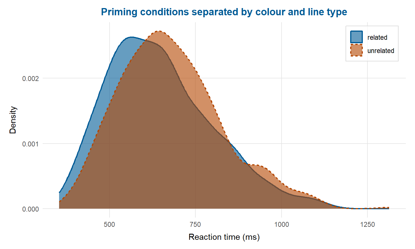
The palette starts from the colours proposed by Okabe and Ito (2008), and colour-vision simulations use the model of Machado et al. (2009). The audit still reports measurements beside thresholds because a journal, display size or printing process may require a different decision.
Limits
depictr draws and checks figures. It does not choose the model, contrasts or prior. A polished plot can faithfully present a poor analysis. The checks also cover measurable properties, not every barrier a reader may face. Alt text, a meaningful caption and a sensible figure order remain editorial work.
The R reference and Python reference cover diagnostics, posterior plots, power curves, model comparisons and multi-panel composition. Their place is in the reference material. The useful habit for an analysis is smaller: use one set of conventions throughout, then audit the exact figure that will leave the project.
References
Machado, G. M., Oliveira, M. M., & Fernandes, L. A. F. (2009). A physiologically-based model for simulation of color vision deficiency. IEEE Transactions on Visualization and Computer Graphics, 15(6), 1291–1298. https://doi.org/10.1109/TVCG.2009.113
Okabe, M., & Ito, K. (2008). Color universal design (CUD): How to make figures and presentations that are friendly to colorblind people. https://jfly.uni-koeln.de/color/ (Original work published 2002)
Comments are provided by Disqus and are not loaded automatically. Loading them connects your browser to Disqus, which may use cookies and process data under its privacy policy. See this site's privacy notice for details.